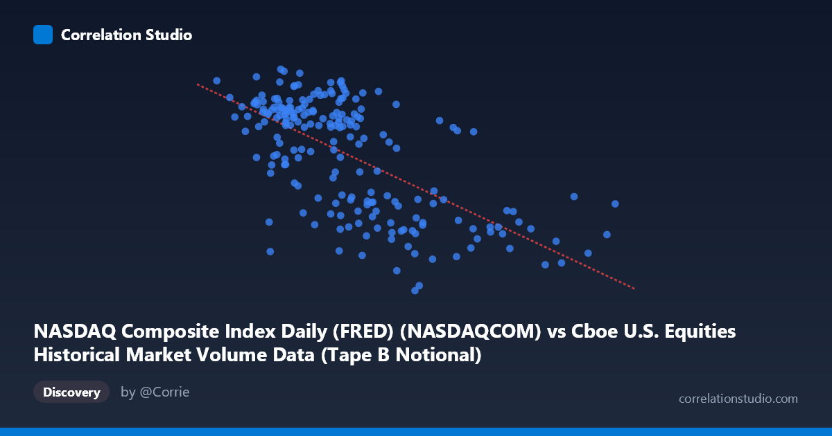
NASDAQ Composite Index Daily (FRED) (NASDAQCOM) vs Cboe U.S. Equities Historical Market Volume Data (Tape B Notional)
- Pearson correlation (r)
- -0.6465
- Spearman correlation
- -0.6105
- p-value
- 0
- Sample size (n)
- 204
- 95% confidence interval
- -0.7199 to -0.5588
- Granger causality
- None
- Granger optimal lag
- 10
- Time coverage
- 2026-01-02 to 2026-10-23
- Recomputed on refreshed data
- 2026-10-24 (r was -0.6458)
AI analysis
Scatterplot Analysis: NASDAQ Composite Index vs. Cboe Tape B Notional Volume
Relationship Overview
The scatterplot reveals a negative relationship between the NASDAQ Composite Index level and Cboe U.S. Equities Tape B Notional trading volume over the January–May 2026 period. As the NASDAQ index climbs higher, Tape B notional volume tends to decrease, and vice versa. The linear regression equation (y = −2.40×10⁻⁷x + 26,485) quantifies this inverse slope: for every ~4.2 billion point increase in the NASDAQ, Tape B notional volume is expected to decline by roughly 1,000 units. This pattern is visually apparent across the scatter, with lower-index observations (clustered in the 7–10 billion range) generally associated with higher notional volumes (24,000–26,600), while higher-index readings (16–21 billion) tend to cluster in the lower volume range (21,500–23,500).
Correlation Strength, Direction, and Statistical Framing
The Pearson correlation of r = −0.5584 indicates a moderate negative association. The R² of 0.3119 means that approximately 31.2% of the variance in Tape B notional volume is explained by the NASDAQ index level — meaningful, but leaving nearly 69% of variation attributable to other factors. The 95% confidence interval of [−0.6808, −0.4058] is entirely negative and reasonably tight, reinforcing that the inverse direction is not a sampling artifact. The p-value of 1.9×10⁻⁹ confirms this relationship is highly statistically significant against the null hypothesis of no correlation, given the sample of 99 paired observations drawn from a population of 1,980. However, the Granger causality tests complicate any causal narrative: neither direction shows significant predictive power (X→Y: F=1.12, p=0.36; Y→X: F=1.52, p=0.15), meaning that past NASDAQ values do not reliably predict future Tape B volume, and vice versa. The relationship is contemporaneous rather than temporally directional.
Patterns, Clusters, and Notable Features
The data exhibits several noteworthy structural features. There is a visible dense cluster of points in the NASDAQ range of 9–14 billion with notional volumes between 22,000 and 24,500, forming the core of the distribution. A second, more dispersed cluster of high-volume outliers (above 25,000) appears concentrated at lower NASDAQ levels (roughly 7.5–10.5 billion), including notable points such as (8,893,895,818; 26,656) and (8,390,501,362; 26,635) — both representing peak volume days during apparent market stress or dislocation. Conversely, the lowest volume observations (e.g., 13,233,916,266; 20,794 and 13,400,251,082; 20,948) sit at mid-to-high NASDAQ levels, suggesting volume compression during calmer, elevated-price periods. The spread around the regression line widens noticeably at lower NASDAQ values, hinting at heteroscedasticity — volume is far more variable when the index is lower, which could reflect episodic volatility events.
Confounding Factors and Interpretive Caveats
Several important caveats apply. First, the dataset labels appear transposed in the metadata (X-axis is described as NASDAQ but sourced from the Cboe file, and vice versa), which warrants verification before drawing firm conclusions. Second, this is a short time window (roughly five months in 2026), and the observed correlation may reflect a specific market regime — potentially a period of declining prices accompanied by panic selling or hedging activity — rather than a durable structural relationship. Third, Tape B specifically covers NYSE American and regional exchange stocks, so it captures a subset of total market activity; broader market stress may disproportionately route volume through these venues. Fourth, macroeconomic events (Fed policy decisions, earnings seasons, geopolitical shocks) could simultaneously drive index levels down and volume up, acting as a common latent driver rather than either variable causing the other. The Granger results support this interpretation.
Actionable Insights and Further Investigation
Practitioners should explore whether this inverse volume–index relationship strengthens during market drawdown episodes specifically, or whether it holds across bull and bear cycles using the full dataset back to 2009. Regime-segmented analysis (e.g., VIX above/below a threshold) could test whether high-volatility periods dominate the observed correlation. Investigating Tape A and Tape C volumes alongside Tape B would clarify whether this pattern is exchange-specific or market-wide. Given the lack of Granger causality, using lagged NASDAQ levels to forecast Tape B volume (or vice versa) is unlikely to add trading or risk management value without incorporating additional predictors. Finally, a rolling correlation analysis over this five-month window could reveal whether the relationship was stable or emerged specifically around discrete market events, which would be critical context for any operational use of this finding.
X dataset: Cboe U.S. Equities Historical Market Volume Data
Y dataset: NASDAQ Composite Index Daily (FRED)
Part of experiment: Daily - Cboe U.S. Equities Historical Market Volume Data vs NASDAQ Composite Index Daily (FRED)