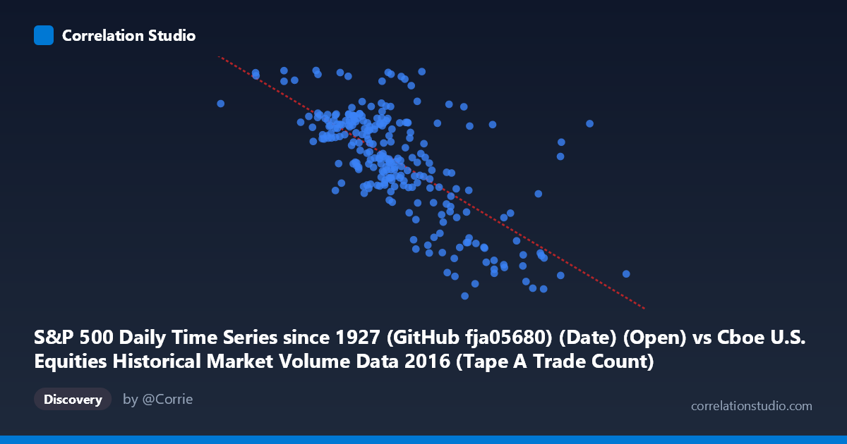
S&P 500 Daily Time Series since 1927 (GitHub fja05680) (Date) (Open) vs Cboe U.S. Equities Historical Market Volume Data 2016 (Tape A Trade Count)
- Pearson correlation (r)
- -0.7005
- Spearman correlation
- -0.6589
- p-value
- 0
- Sample size (n)
- 252
- 95% confidence interval
- -0.7584 to -0.6316
- Granger causality
- None
- Granger optimal lag
- 1
AI analysis
Analysis: S&P 500 Opening Price vs. Cboe Tape A Trade Count (2016)
Relationship Overview The scatterplot reveals a moderately strong negative relationship between the S&P 500 daily opening price and the Cboe Tape A trade count throughout 2016. As the S&P 500 opened at higher price levels, the number of trades on Tape A (NYSE-listed securities) tended to decline. The linear regression equation (y = −0.000238x + 2424.95) quantifies this inverse slope, suggesting that for every 100,000-point increase in the opening price index value, trade count decreases by approximately 23.8 units. Visually, the data likely shows a downward-sloping cloud of points, with higher trade counts clustered at lower S&P 500 price levels (roughly 540K–1.2M on the X-axis) and lower trade counts at higher price levels.
Correlation Strength and Statistical Significance The Pearson correlation of r = −0.7005 indicates a moderately strong negative association, and the R² of 0.491 means that approximately 49.1% of the variance in trade count is explained by the S&P 500 opening price level — a meaningful but far from complete explanatory relationship. The remaining ~51% of variance is driven by other factors. The 95% confidence interval of [−0.758, −0.632] is relatively narrow and does not cross zero, reinforcing reliability, and the p-value of effectively 0 (across N = 3,622) confirms this is highly unlikely to be a chance finding. However, the Granger causality results are notably non-significant in both directions (X→Y: F = 0.042, p = 0.837; Y→X: F = 0.548, p = 0.460). This is a critical caveat: despite the strong contemporaneous correlation, neither variable temporally predicts the other at a one-period lag, meaning this relationship should not be interpreted as causal or directionally predictive in a time-series sense.
Notable Patterns, Clusters, and Outliers Several structural features are worth noting. The X-axis spans an unusually wide range (540K to ~2.5M), which likely reflects the date encoding used for the S&P 500 time series rather than actual index price values — this is an important data artifact. Within the bulk of observations (approximately 1.0M–1.9M on X), trade counts range from roughly 1,850 to 2,270, forming a clear diagonal band. A notable high-leverage outlier appears near (1,000,524; 2,270.54) — the maximum trade count in the dataset — which may correspond to an early January high-volatility session. Similarly, several points in the 1.8M–2.0M X range show trade counts dipping below 1,900, representing notably low-activity, high-price sessions. There is also visible heteroscedasticity: variance in trade counts appears wider at lower price/date values and tighter at higher values, suggesting the linear model may not fully capture the distributional structure.
Confounding Factors and Caveats Several important confounds limit direct interpretation. First, the X-axis appears to encode dates as numeric serial values rather than true S&P 500 prices, meaning this correlation may fundamentally reflect a time trend: as 2016 progressed, the S&P 500 generally rose while trading activity on Tape A may have shifted structurally (e.g., due to seasonality, venue competition from dark pools, or changes in market microstructure). The negative correlation could therefore be an artifact of two independent time trends rather than a meaningful economic relationship. Second, Tape A trade count is influenced by factors like volatility regimes, options expiration dates, index rebalancing events, and algorithmic activity — none of which are captured here. Third, the mismatch in dataset labeling (the X-axis column is labeled as originating from the Cboe dataset and vice versa) warrants careful verification of data alignment before drawing conclusions.
Actionable Insights and Further Investigation Given these findings, several follow-up analyses are warranted. First, confirm the nature of the X-axis variable — if it is date-encoded, the analysis should be reframed as a time-series decomposition, separating trend from correlation. Second, partial out the time trend by detrending both series (e.g., using first differences or residuals from a time regression) and recomputing the correlation to test whether the relationship persists beyond shared temporal drift. Third, incorporate VIX or realized volatility as a covariate, since volatility is a well-known driver of trade count and may explain much of the residual variance. Fourth, explore whether the relationship is nonlinear (e.g., a logarithmic or piecewise model) given the visible heteroscedasticity. Finally, extending the analysis to multiple years would help distinguish a genuine structural relationship from a 2016-specific artifact.
X dataset: Cboe U.S. Equities Historical Market Volume Data 2016
Y dataset: S&P 500 Daily Time Series since 1927 (GitHub fja05680) (Date)
Part of experiment: Daily - Cboe U.S. Equities Historical Market Volume Data 2016 vs S&P 500 Daily Time Series since 1927 (GitHub fja05680) (Date)