World Bank CO2 Emissions by Country (DataBank) (Bunker fuels (Not in Total)) vs US Employment and Unemployment (employed_total)
- Pearson correlation (r)
- 0.9497
- Spearman correlation
- 0.9713
- p-value
- 0
- Sample size (n)
- 80
- 95% confidence interval
- 0.9225 to 0.9675
- Granger causality
- None
- Granger optimal lag
- 10
AI analysis
Analysis: Bunker Fuel CO₂ Emissions vs. US Total Employment (1941–2020)
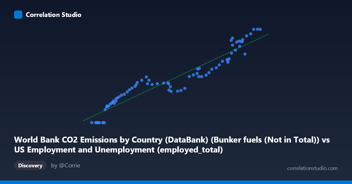
1. Relationship Overview The scatterplot reveals a strong, positive, and largely linear relationship between global bunker fuel CO₂ emissions (X-axis) and US total employment (Y-axis) across eight decades of annual observations. As bunker fuel emissions increase from roughly 50,000 to 157,000 (units), US total employment rises from near zero (relative baseline) to approximately 1,591 (thousands or millions). The linear regression equation ŷ = 0.0125x − 529.71 fits the data well visually, with points clustering tightly around the regression line across most of the range, suggesting a remarkably consistent co-movement between these two variables over time.
2. Correlation Strength, Direction, and Causality The Pearson correlation of r = 0.9497 indicates a very strong positive association, and the R² = 0.902 means that approximately 90.2% of the variance in US total employment is statistically explained by variation in bunker fuel emissions within this paired sample — an unusually high figure for two seemingly disparate datasets. The 95% confidence interval for r of [0.923, 0.968] is narrow and entirely positive, confirming the robustness of this association with high certainty, and the p-value of ~0 eliminates any possibility of chance correlation at conventional significance thresholds. However, the Granger causality analysis tells a critically important story: neither direction (X→Y: F = 1.97, p = 0.058; Y→X: F = 1.62, p = 0.129) reaches statistical significance at the α = 0.05 level, even at an optimal lag of 10 periods. This means that neither variable temporally predicts the other beyond baseline trends — a strong signal that the correlation reflects shared common drivers rather than any mechanistic causal pathway between bunker fuel emissions and US employment.
3. Notable Patterns, Clusters, and Outliers Several observations stand out structurally. At the lower end of X (roughly 50,000–65,000), a cluster of points shows Y values of exactly 0.00 for multiple observations — these likely represent the earliest years of the time series (early 1940s) where employment data may be missing, censored, or defined differently, and they form a somewhat anomalous horizontal band along the X-axis that slightly distorts the linear fit. The middle range (80,000–130,000) shows the densest clustering with moderate scatter, suggesting some variability in the employment-emissions relationship during mid-century economic cycles (recessions, expansions). At the upper end (140,000–157,000), points again cluster tightly near the regression line with high Y values, consistent with the post-2000 era of globalized trade and high employment. There are no dramatic single-point outliers, but the zero-Y cluster at low X deserves methodological scrutiny.
4. Confounding Factors and Interpretive Caveats This correlation is almost certainly a classic spurious correlation driven by shared temporal trends — both variables are non-stationary time series that trend upward over the 1941–2020 period due to global economic growth, population expansion, and post-WWII industrialization. Any two variables that both trend upward over 80 years will exhibit high correlation without meaningful causal linkage. The dataset labeling also raises concerns: the X-axis column is described as sourced from "US Employment and Unemployment" data while measuring CO₂ bunker fuels, and the Y-axis is labeled as from "World Bank CO₂" data while measuring US employment — suggesting possible dataset join or labeling artifacts that warrant verification. Additionally, bunker fuels (international shipping and aviation) are explicitly "not included in national totals," making any direct policy or economic link to domestic US employment particularly tenuous.
5. Actionable Insights and Further Investigation Given the high R² but absent Granger causality, the priority recommendation is to detrend both time series (e.g., via first-differencing or HP filtering) before drawing any conclusions — if the correlation collapses after detrending, it confirms spuriousness. Researchers should also verify the dataset join logic, as the cross-labeled sources suggest a potential data pipeline error. Further investigation could examine whether the relationship holds during specific economic shocks (2008–2009 financial crisis, COVID-19 2020) where both series would be expected to drop simultaneously — such co-movement during shocks would be more economically meaningful than the long-run trend correlation. Finally, introducing GDP as a control variable in a multivariate regression would help isolate whether any residual relationship between bunker emissions and employment persists once the dominant common driver (economic output) is accounted for.
X dataset: US Employment and Unemployment
Y dataset: World Bank CO2 Emissions by Country (DataBank)
Part of experiment: Yearly - US Employment and Unemployment vs World Bank CO2 Emissions by Country (DataBank)