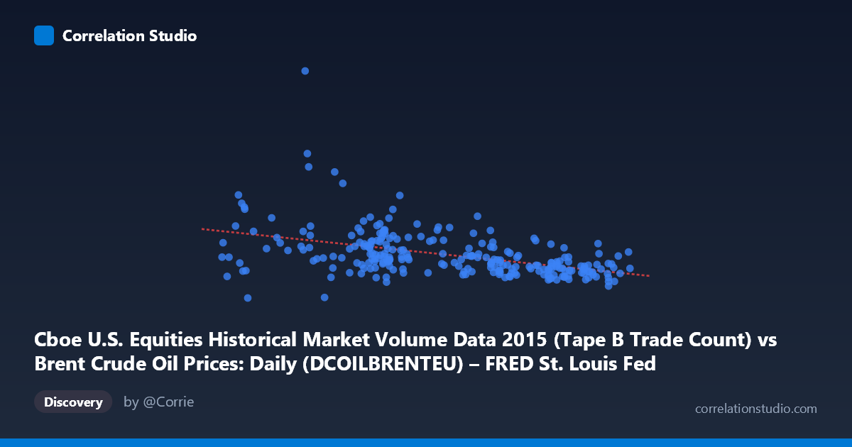
Cboe U.S. Equities Historical Market Volume Data 2015 (Tape B Trade Count) vs Brent Crude Oil Prices: Daily (DCOILBRENTEU) – FRED St. Louis Fed (DCOILBRENTEU)
- Pearson correlation (r)
- -0.4573
- Spearman correlation
- -0.516
- p-value
- 0
- Sample size (n)
- 251
- 95% confidence interval
- -0.55 to -0.3535
- Granger causality
- None
- Granger optimal lag
- 10
AI analysis
Scatterplot Analysis: Brent Crude Oil Price vs. Cboe Tape B Trade Count (2015)
Relationship Overview
The scatterplot reveals a negative relationship between daily Brent crude oil prices (X-axis) and Cboe Tape B trade counts (Y-axis) across 2015. The linear regression equation (y = −5,352.37x + 579,091) confirms that as oil prices increase, trade counts tend to decrease. This inverse pattern is visually apparent in the downward-sloping trend, though the scatter is substantial, indicating the relationship is far from deterministic. The data spans the full calendar year 2015, a period during which Brent crude experienced notable price volatility, declining from higher levels earlier in the year toward multi-year lows, which likely contributes to the dynamic range captured here.
Correlation Strength, Direction, and Statistical Significance
The Pearson correlation of r = −0.457 reflects a moderate negative association, but the more practically informative metric is R² = 0.209 — meaning oil prices explain only about 20.9% of the variance in Tape B trade counts. The remaining ~79% is driven by factors entirely outside this relationship. The 95% confidence interval of [−0.550, −0.354] is reasonably tight and sits entirely below zero, providing strong statistical confidence that the negative direction is genuine rather than artifactual. The p-value of 2.24 × 10⁻¹⁴ confirms the correlation is highly statistically significant given the sample (n = 251). However, the Granger causality results are unambiguous in their null finding: neither X→Y (F = 0.613, p = 0.802) nor Y→X (F = 0.717, p = 0.708) reached significance at an optimal lag of 10 periods. This means that past oil prices do not temporally predict future trade counts, and vice versa — the correlation is contemporaneous and associative, not predictive in a directional, time-lagged sense.
Notable Patterns, Clusters, and Outliers
Several structural features stand out in the data. There is a visible cluster of high trade-count observations (Y 450,000–600,000+) concentrated in the lower oil price range (roughly X = 36–50), consistent with the negative slope. However, this region also exhibits enormous vertical spread — for instance, observations near X ≈ 44–48 show trade counts ranging from roughly 210,000 to over 620,000, suggesting high conditional variance. A few notable high-leverage outliers are present: points near (43.84, 621,009) and (41.86, 640,679) represent unusually high trade volumes at low oil prices and may disproportionately influence the regression slope. Conversely, at higher oil prices (X 60), the data compresses into a relatively narrow Y-band (~176,000–365,000), suggesting less volatility in trading activity when prices are elevated. One point near (48.27, 474,961) and (48.80, 529,371) also appears elevated relative to its neighbors. There is also a possible non-linear feature — the relationship may be stronger at the lower price tail and flatter in the mid-range, hinting that a logarithmic or piecewise model might outperform the linear fit.
Confounding Factors and Interpretive Caveats
Several important caveats temper interpretation. First, the axis labels appear to be swapped in the dataset metadata — the X-axis is labeled as the Brent crude price column from the Cboe dataset, and the Y-axis as the trade count column from the FRED dataset, which is counter-intuitive and should be verified before drawing conclusions. Second, the year 2015 was an exceptional period for both oil markets (sharp price declines driven by OPEC supply decisions) and equity markets (August 2015 volatility spike), meaning both variables were simultaneously responding to macro shocks — classic confounding by common cause. Global risk sentiment, USD strength, and Federal Reserve policy all moved both oil prices and equity trading volumes in 2015 independently. Third, Tape B specifically covers regional exchange volume (BATS/EDGA/EDGX), which may reflect fragmentation dynamics and algorithmic routing behavior rather than fundamental market interest in oil. Fourth, the Granger null result strongly cautions against interpreting the correlation as any form of leading indicator relationship between these series.
Actionable Insights and Further Investigation
Despite the correlation's limitations, several avenues are worth pursuing. Analysts should control for common macro drivers — particularly VIX, USD index (DXY), and S&P 500 returns — using a multivariate regression or partial correlation to isolate whether oil prices retain independent explanatory power over Tape B volumes. The outlier points (notably the two observations exceeding 600,000 trades at sub-44 price levels) deserve date-specific investigation to determine whether they coincide with identifiable market events such as the August 2015 flash crash or OPEC announcements. Exploring a non-linear model (e.g., log-linear or polynomial regression) could meaningfully improve on the 20.9% R² given the apparent heteroscedasticity. Finally, extending the analysis to multiple years (2014–2016) would test whether the 2015 negative correlation is structurally persistent or an artifact of that year's unusual commodity and equity market conditions.
X dataset: Brent Crude Oil Prices: Daily (DCOILBRENTEU) – FRED St. Louis Fed
Y dataset: Cboe U.S. Equities Historical Market Volume Data 2015
Part of experiment: Daily - Brent Crude Oil Prices: Daily (DCOILBRENTEU) – FRED St. Louis Fed vs Cboe U.S. Equities Historical Market Volume Data 2015