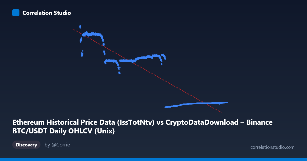
Ethereum Historical Price Data (IssTotNtv) vs CryptoDataDownload – Binance BTC/USDT Daily OHLCV (Unix)
- Pearson correlation (r)
- -0.8919
- Spearman correlation
- -0.7251
- p-value
- 0
- Sample size (n)
- 3191
- 95% confidence interval
- -0.8988 to -0.8846
- Granger causality
- None
- Granger optimal lag
- 10
AI analysis
Analysis: Time vs. Ethereum-Labeled Metric
Important preliminary note: The X-axis is labeled as a timestamp (Unix time, spanning 2017–2026), yet described as "Ethereum Historical Price Data." The Y-axis is labeled "Binance BTC/USDT Daily OHLCV." This suggests the axis labels/descriptions may be swapped or mismatched in the dataset metadata — what's actually being analyzed appears to be a time-series trend, not a direct relationship between two independent financial variables. This should be clarified before drawing substantive conclusions.
1. What the Visualization Reveals
Treating X as time and Y as a price-like metric, the data shows a strong declining trend over the ~9-year window. Sample points confirm this: early observations (2017–2018) cluster around 18,000–21,000, mid-period values (2020–2022) sit near 13,000–14,900, and recent/future-dated points (2023–2026) drop sharply to 1,600–2,800. This is not a smooth linear decay but appears to occur in distinct regime plateaus — suggesting structural breaks or regime shifts rather than continuous drift.
2. Strength, Direction, and Statistical Confidence
- r = -0.892, r² = 0.796: A strong negative relationship exists, with time (or the X-variable) explaining ~80% of the variance in Y. This is a substantial fit for real-world financial/time data, though 20% remains unexplained — likely due to the regime-like clustering rather than pure linear decay. - 95% CI [-0.899, -0.885]: Very tight interval given the large sample (n=3,191), indicating high precision in the correlation estimate. - p ≈ 0: The relationship is highly statistically significant — essentially no chance this is due to random noise, though with financial time series, autocorrelation inflates apparent significance. - Granger causality: Neither direction shows significant causality (X→Y: p=0.636; Y→X: p=0.078, borderline but not significant at 0.05). This is critical — the strong correlation does NOT imply predictive causality. If X is genuinely a time index, Granger causality is somewhat meaningless in this framing (time doesn't "cause" in the Granger sense), reinforcing that this is a trend/level relationship, not a dynamic predictive one.
3. Notable Patterns and Non-linearities
The sampled data reveals at least 3-4 distinct value clusters rather than smooth linear decline: - ~18,500–21,000 (2017–2018 points) - ~13,300–14,900 (2019–2023 points, a long plateau) - ~1,600–2,800 (2023–2026 points, a sharp drop)
This step-like structure suggests regime changes (e.g., market cycle shifts, bear markets, or a structural break in whatever process generated Y) rather than continuous decay — the linear model captures the broad negative slope but likely underfits the actual step-function-like behavior, explaining why 20% of variance remains unexplained despite high significance.
4. Caveats and Confounders
- Label ambiguity: The mismatched axis descriptions (Ethereum vs. BTC/USDT) must be resolved — this analysis may actually reflect a mislabeled single-asset time series rather than an X-Y relationship between two distinct crypto assets. - Autocorrelation: Both variables (especially if genuinely time-indexed price series) violate independence assumptions, inflating the statistical significance (p≈0) beyond what's practically meaningful. - Non-stationarity: Financial time series with strong trends often show spurious correlations with any monotonic variable, including time itself. - Future-dated data: X values extend to 2026, beyond the current date — verify whether these are forecasts, placeholder values, or data entry errors.
5. Recommended Next Steps
1. Clarify data labels — confirm which variable is actually price vs. time/index before further modeling. 2. Test for structural breaks (e.g., Chow test, Bai-Perron) given the visible plateau pattern rather than assuming pure linearity. 3. Difference or detrend the series and re-run correlation/Granger tests on stationary transformations to check if the relationship holds beyond shared trend. 4. Segment analysis by regime (2017–18, 2019–22, 2023–26) to model each cluster separately, likely improving fit beyond the 79.6% linear R².
X dataset: CryptoDataDownload – Binance BTC/USDT Daily OHLCV
Y dataset: Ethereum Historical Price Data
Part of experiment: Bitcoin - CryptoDataDownload – Binance BTC/USDT Daily OHLCV vs Ethereum Historical Price Data