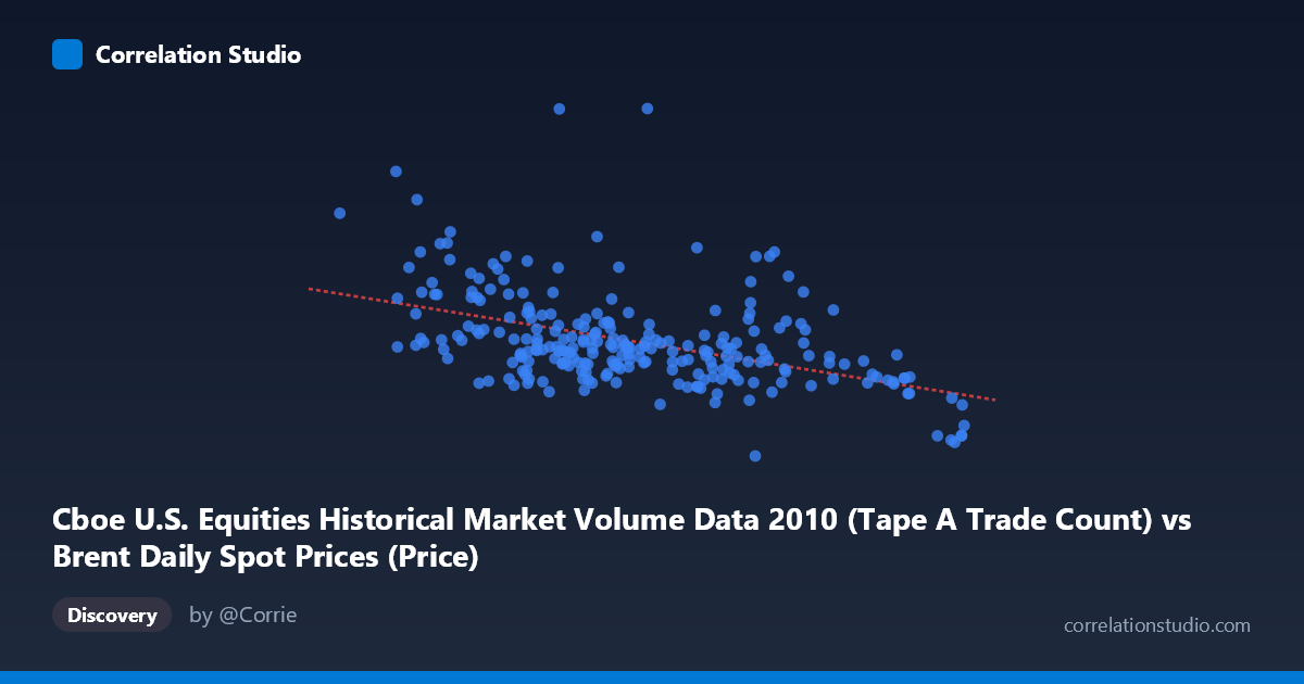
Cboe U.S. Equities Historical Market Volume Data 2010 (Tape A Trade Count) vs Brent Daily Spot Prices (Price)
- Pearson correlation (r)
- -0.468
- Spearman correlation
- -0.4619
- p-value
- 0
- Sample size (n)
- 252
- 95% confidence interval
- -0.5592 to -0.3655
- Granger causality
- None
- Granger optimal lag
- 10
AI analysis
Analysis: Brent Crude Oil Prices vs. U.S. Equity Trade Count (2010)
Relationship Overview The scatterplot reveals a moderate negative relationship between Cboe U.S. equity trade counts (X-axis, measured in tape A trades) and Brent crude oil spot prices (Y-axis, in USD/barrel) across 252 trading days in 2010. As equity market trade volume increases, Brent crude prices tend to decline — a counterintuitive finding at first glance, but one that reflects the complex interplay between equity market activity and commodity pricing during this post-financial-crisis period. The linear regression equation (y = -31,266.7x + 3,805,530) quantifies this inverse slope, suggesting that each unit increase in trade count is associated with a decrease of roughly 31,267 units in crude price, though the practical interpretation requires careful framing given the dataset's characteristics.
Correlation Strength and Statistical Significance The Pearson correlation of r = -0.468 indicates a moderate negative association, but the explanatory power is modest: R² = 0.219, meaning only about 21.9% of the variance in Brent crude prices is explained by equity trade count. The remaining ~78% is attributable to other factors entirely. The 95% confidence interval of [-0.559, -0.366] is comfortably away from zero, and the p-value of 3.997 × 10⁻¹⁵ is highly significant given N = 3,302 and n = 252 — so this is not a noise artifact. However, statistical significance here is partly a function of the large population size, and should not be conflated with practical or economic significance. Critically, Granger causality tests show no significant predictive directionality in either direction (X→Y: F = 0.899, p = 0.535; Y→X: F = 0.857, p = 0.575) at the optimal lag of 10 periods. This means that neither variable reliably predicts the other temporally — the correlation is contemporaneous and associative, not predictively causal.
Notable Patterns, Clusters, and Outliers Several features stand out in the sample points. There is a visible cluster of moderate trade counts (75–82 range) paired with mid-range oil prices (roughly 1,000,000–1,400,000 units), forming the dense core of the distribution. However, notable outliers distort the picture significantly: the point at (76.48, 3,216,587) represents an extreme high-price observation at a relatively average trade count, likely corresponding to a specific market event. Similarly, (70.45, 2,474,888) and (71.43, 2,114,898) show that lower trade counts are associated with some of the highest price readings, consistent with the negative trend. At the high-trade-count extreme, (93.63, 627,720) and (93.55, 796,428) anchor the lower-right of the plot. The relationship also appears to carry non-linear characteristics — the spread in Y values is substantially wider at lower X values, suggesting possible heteroscedasticity and that a simple linear model may be underfitting the true relationship.
Confounding Factors and Caveats This correlation almost certainly reflects shared macroeconomic dynamics rather than any direct causal link between equity trading volume and crude oil pricing. In 2010, markets were recovering from the 2008–2009 financial crisis, and periods of risk-off sentiment (lower equity trading activity, higher commodity prices driven by inflation hedging or supply concerns) versus risk-on sentiment (higher trading volumes, calmer commodity markets) could produce exactly this inverse pattern as a spurious byproduct. The dataset mismatch is also notable — the X variable is labeled as coming from a "Brent Daily Spot Prices" dataset while the Y variable comes from a "Cboe Market Volume" dataset, suggesting possible column assignment confusion that warrants verification. Additionally, crude oil prices in 2010 were influenced by OPEC decisions, the Deepwater Horizon spill, and dollar strength, none of which are captured here.
Actionable Insights and Further Investigation Given the lack of Granger causality, trading strategies based on this relationship should not assume predictive power — the correlation is contemporaneous at best. Further investigation should include: (1) introducing a common macro factor such as the VIX, USD index, or S&P 500 returns to test whether this correlation disappears as a confound; (2) testing non-linear models (e.g., polynomial or spline regression) given the apparent heteroscedasticity at low trade counts; (3) verifying the dataset column assignments to ensure X and Y represent what is claimed; and (4) extending the time series beyond 2010 to test whether this negative correlation is structural or specific to the post-crisis recovery environment. A partial correlation analysis controlling for macroeconomic conditions would likely substantially reduce or eliminate the observed r = -0.468.
X dataset: Brent Daily Spot Prices
Y dataset: Cboe U.S. Equities Historical Market Volume Data 2010
Part of experiment: Daily - Brent Daily Spot Prices vs Cboe U.S. Equities Historical Market Volume Data 2010