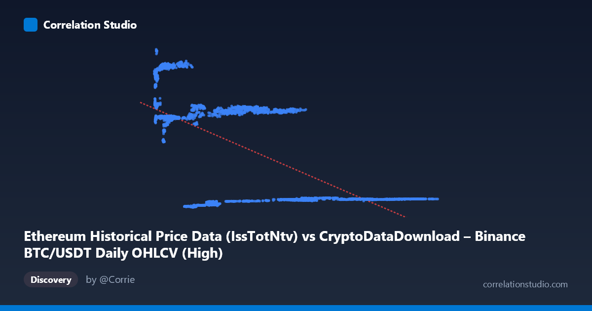
Ethereum Historical Price Data (IssTotNtv) vs CryptoDataDownload – Binance BTC/USDT Daily OHLCV (High)
- Pearson correlation (r)
- -0.6385
- Spearman correlation
- -0.4698
- p-value
- 0
- Sample size (n)
- 3191
- 95% confidence interval
- -0.6586 to -0.6174
- Granger causality
- Y → X
- Granger optimal lag
- 10
AI analysis
Scatterplot Analysis: X-axis Metric vs. Y-axis Metric
1. Overall Relationship Pattern
The scatterplot reveals a clear negative, non-linear relationship between the two variables. Rather than a smooth linear decline, the data appears organized into distinct horizontal bands or clusters — for example, groups of points clustering around Y≈2,400–2,800, Y≈13,400–14,900, and Y≈18,500–21,000, each spanning a fairly wide range of X values. This banding suggests the relationship may be episodic or regime-based rather than continuously proportional — consistent with time-series data (likely price data) that moves through distinct market phases rather than following a steady functional trend.
2. Correlation Strength, Direction & Statistical Confidence
The correlation coefficient (r = -0.6385) indicates a moderate-to-strong negative association, but R² = 0.4076 tells the more important story: only about 41% of the variance in Y is explained by X, leaving roughly 59% driven by other factors or noise. The 95% CI [-0.6586, -0.6174] is tight and does not cross zero, and the p-value of 0 confirms this negative relationship is highly statistically significant — but statistical significance here reflects the large sample size (n=3,191) more than practical predictive power, given the moderate R².
The Granger causality results add an important temporal dimension: Y Granger-causes X (unidirectional), with a significant lag-10 relationship (F=1.93, p=0.037) in the Y→X direction, while X→Y shows no significant predictive power (p=0.786). This suggests that past values of Y (Ethereum price/native units) help predict future X (BTC/USDT price) at a ~10-day lag, but the reverse is not supported. This is a meaningful asymmetry: the correlation alone doesn't establish direction, but the Granger test suggests ETH-related movements may lead BTC movements, not vice versa.
3. Notable Patterns and Outliers
The clustering is the most striking feature — the data doesn't fill the scatter space smoothly but occupies discrete "shelves." This is typical of cryptocurrency price series with distinct historical regimes (e.g., 2018 bear market, 2020–21 bull run, 2022 crash), where both BTC and ETH prices moved through correlated but choppy phases. There also appears to be a dense low-Y, wide-X band (Y≈2,300–2,900 across X from ~20,000 to over 100,000), suggesting one asset (likely BTC in USDT terms) reached very high price levels while the other metric (possibly ETH issuance/native units) stayed compressed — hinting at a supply-vs-price or unit-scale mismatch rather than a pure price-price relationship.
4. Confounding Factors and Caveats
Because this spans 2017–2026, both series are subject to shared macro crypto-market cycles (bull/bear regimes, halving events, regulatory shocks) that could drive spurious correlation without direct causal linkage. Additionally, the X-axis label ("IssTotNtv" — issuance in native units) and Y-axis label (BTC/USDT High price) suggest these may be mismatched units/scales (a supply metric vs. a price metric), which complicates interpretation — the negative correlation could reflect a supply-and-demand relationship, general crypto-market inverse cycles, or simply autocorrelated time trends in two non-stationary series. Time-series data like this often violates the i.i.d. assumptions behind standard correlation/significance tests, inflating apparent significance.
5. Recommendations for Further Investigation
1. Verify axis definitions — clarify whether X is truly issuance and Y is truly BTC price; a supply-price relationship warrants very different economic interpretation than two price series. 2. Test for stationarity (ADF/KPSS) and consider differencing or log-returns before correlation/Granger analysis, since raw price/issuance levels are likely non-stationary and can produce misleading causality results. 3. Segment by market regime (bull/bear/sideways) to see if the negative correlation holds within each cluster or is purely an artifact of regime-switching. 4. Explore the 10-day lag mechanism — investigate what economic mechanism would cause Y to lead X, and test robustness with alternate lag structures. 5. Control for shared market factors (e.g., overall crypto market cap, USD liquidity) via partial correlation or multivariate models to isolate the genuine bilateral relationship from broader macro co-movement.
X dataset: CryptoDataDownload – Binance BTC/USDT Daily OHLCV
Y dataset: Ethereum Historical Price Data
Part of experiment: Bitcoin - CryptoDataDownload – Binance BTC/USDT Daily OHLCV vs Ethereum Historical Price Data