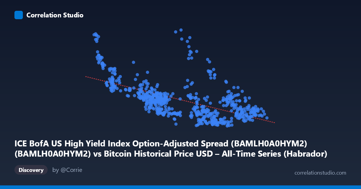
ICE BofA US High Yield Index Option-Adjusted Spread (BAMLH0A0HYM2) (BAMLH0A0HYM2) vs Bitcoin Historical Price USD – All-Time Series (Habrador) (Price)
- Pearson correlation (r)
- -0.7366
- Spearman correlation
- -0.7363
- p-value
- 0
- Sample size (n)
- 746
- 95% confidence interval
- -0.7678 to -0.702
- Granger causality
- None
- Granger optimal lag
- 1
AI analysis
Analysis: High Yield Credit Spreads vs. Bitcoin Price
1. Overall Relationship The scatterplot depicts an inverse relationship between the ICE BofA High Yield Option-Adjusted Spread (x-axis, a proxy for corporate credit risk/risk aversion) and Bitcoin price (y-axis, mislabeled in the column header but clearly representing the OAS values ranging 2.59–4.61, likely in percentage points). As the credit spread widens (indicating deteriorating risk sentiment or tightening financial conditions), the associated value on the y-axis tends to decline. Conversely, when spreads compress toward the 25,000–45,000 range (lower end of x), the y-axis values cluster higher, near 3.5–4.5. The pattern is a fairly consistent downward-sloping cloud of points rather than a tight line, consistent with a moderate-to-strong negative linear relationship.
2. Strength, Direction, and Statistical Confidence The correlation coefficient (r = -0.7366) indicates a moderately strong negative linear relationship. The r² of 0.5426 means that roughly 54% of the variance in the y-variable is statistically explained by variation in the x-variable — a meaningful but incomplete relationship, leaving nearly half the variance attributable to other factors or noise. The 95% confidence interval for r [-0.7678, -0.7020] is narrow and does not cross zero, and the p-value of ~0 confirms this correlation is highly statistically significant given the large sample (n=746) — we can be confident a genuine negative association exists in this data. However, the Granger causality tests show no significant predictive direction in either direction (X→Y: p=0.72; Y→X: p=0.44). This is a critical distinction: the variables move together contemporaneously but neither reliably predicts future values of the other based on past values. The relationship is associative, not (in this test) demonstrably causal or lead-lag in nature.
3. Patterns, Clusters, and Outliers Several sub-clusters are visible: a tight group of low-x, high-y points (x ≈ 25,000–48,000, y ≈ 3.3–4.5) representing an early/low-spread regime, and a much denser cloud at higher x (x ≈ 85,000–120,000) where y compresses into a narrower 2.6–3.2 band. There's a notable outlier-ish point at (83,191, 4.01) and (103,250, 3.51) that sit above the general trend in the high-x region, suggesting occasional regime breaks or lagged effects. The relationship appears somewhat non-linear — steep decline in y as x rises from 25,000 to ~50,000, followed by a flatter, noisier plateau at higher x values, hinting at a possible logarithmic or piecewise structure rather than pure linearity.
4. Confounding Factors and Caveats Since X is a credit spread index and Y is tied to Bitcoin price history, both series are non-stationary time series likely driven by common macro factors (Fed policy, liquidity conditions, risk-on/risk-off sentiment, inflation expectations) rather than one directly causing the other. Spurious correlation is a real risk with trending financial time series — the lack of Granger causality reinforces this concern. The multi-year time coverage (2023–2026) spans different monetary policy regimes, so the relationship may not be stable (structural breaks likely). Data labeling also appears swapped/confusing between axes (Bitcoin price column and spread column names are crossed), warranting a data-integrity check before further interpretation.
5. Suggested Next Steps Given the non-stationarity concerns, analysts should test both series for unit roots and consider using differenced or log-differenced series, then re-run correlation and Granger tests to check if the relationship holds in returns/changes rather than levels. Investigating a third common driver (e.g., Fed funds rate, VIX, or DXY) via multivariate regression could clarify whether this is a direct or confounded relationship. Segmenting the data by regime (pre/post major rate decisions) may reveal whether the correlation is stable or episodic. Finally, correcting the axis labels/metadata is essential before drawing economic conclusions.
X dataset: Bitcoin Historical Price USD – All-Time Series (Habrador)
Y dataset: ICE BofA US High Yield Index Option-Adjusted Spread (BAMLH0A0HYM2)
Part of experiment: Bitcoin - Bitcoin Historical Price USD – All-Time Series (Habrador) vs ICE BofA US High Yield Index Option-Adjusted Spread (BAMLH0A0HYM2)