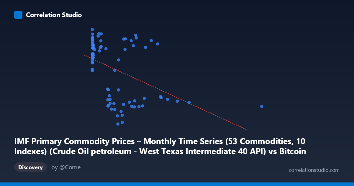
IMF Primary Commodity Prices – Monthly Time Series (53 Commodities, 10 Indexes) (Crude Oil petroleum - West Texas Intermediate 40 API) vs Bitcoin Historical Price USD – All-Time Series (Habrador) (Price)
- Pearson correlation (r)
- -0.4501
- Spearman correlation
- -0.3834
- p-value
- 0.00002
- Sample size (n)
- 83
- 95% confidence interval
- -0.6068 to -0.2596
- Granger causality
- None
- Granger optimal lag
- 1
- Time coverage
- 2010-08-01 to 2017-06-01
- Recomputed on refreshed data
- 2026-10-24 (r was -0.4501)
AI analysis
Analysis: Oil Prices vs. Bitcoin Price
1. What the Visualization Reveals
The scatterplot shows a moderate negative relationship between crude oil (WTI) prices and Bitcoin prices during this 2010–2017 window. Notably, the data is heavily clustered at low oil price values (under ~250), where Bitcoin prices span the full range from ~30 to ~110. As oil prices increase beyond 500–1000+ (units appear to be an unusual scale, possibly indexed or mislabeled), Bitcoin prices consistently sit in the lower range (40–60), creating the visual impression of a downward-sloping trend.
2. Strength, Direction, and Statistical Confidence
The correlation coefficient (r = -0.45) indicates a moderate negative linear relationship, but r² = 0.2025 tells the more important story: only about 20% of the variance in Bitcoin price is explained by oil price movements, leaving 80% attributable to other factors. The 95% CI [-0.61, -0.26] excludes zero and is reasonably tight, and the p-value (1.97E-05) confirms this correlation is statistically significant and unlikely due to chance — but statistical significance here reflects a real but weak-to-moderate association, not a strong predictive relationship. Critically, the Granger causality tests show no significant predictive direction in either direction (X→Y: p=0.166; Y→X: p=0.239). This means neither variable reliably predicts future movements in the other based on past values — the correlation is contemporaneous/coincidental in trend, not causal or forecastable.
3. Notable Patterns and Outliers
The data reveals a clear non-linear, possibly threshold-like structure rather than a clean linear trend. Most low-oil-price points (X < 20) show high Bitcoin prices (85–110), suggesting this cluster corresponds to Bitcoin's earliest history (2010–2012) when prices were low in absolute USD but high on this particular Y-axis scale — likely reflecting index-normalized values. Mid-range X values (200–800) show a bifurcated pattern: some points cluster low (40–60) and others high (95–105), suggesting at least two distinct regimes or time periods are being conflated. The extreme outlier at X=2452.18 (Y=45.17) sits far from the rest of the distribution and may be exerting disproportionate leverage on the regression slope.
4. Confounding Factors and Caveats
This correlation is almost certainly confounded by time — both series exhibit strong secular trends over 2010–2017 independent of each other. Bitcoin experienced massive appreciation and volatility driven by adoption, exchange launches, and speculation, while oil prices were driven by OPEC decisions, US shale production, and global demand shifts (including the 2014–2016 oil price collapse). Any apparent relationship may simply reflect two unrelated trends evolving over the same calendar period rather than genuine economic linkage. Additionally, the small sample size (n=83) relative to the full population (N=449) and the non-linear clustering suggest the linear r² may understate or misrepresent the true relationship shape. Bitcoin's known volatility clustering and regime changes (bubble/crash cycles) also violate typical assumptions of linear correlation analysis.
5. Suggestions for Further Investigation
Rather than relying on raw price correlation, analysts should: (1) test correlations on log-returns or percentage changes rather than price levels, which better isolates genuine co-movement from shared trends; (2) include time as an explicit control variable or use detrended/differenced series; (3) segment the analysis by distinct market regimes (e.g., pre-2013 bubble, 2014 oil crash, 2017 Bitcoin bull run) to check whether the relationship is stable or artifact of specific periods; and (4) explore non-linear or threshold models given the clustered, bifurcated pattern observed. Given the lack of Granger causality, this pairing is not suitable for predictive trading strategies without further transformation of the data.
X dataset: Bitcoin Historical Price USD – All-Time Series (Habrador)
Y dataset: IMF Primary Commodity Prices – Monthly Time Series (53 Commodities, 10 Indexes)
Part of experiment: Bitcoin - Bitcoin Historical Price USD – All-Time Series (Habrador) vs IMF Primary Commodity Prices – Monthly Time Series (53 Commodities, 10 Indexes)