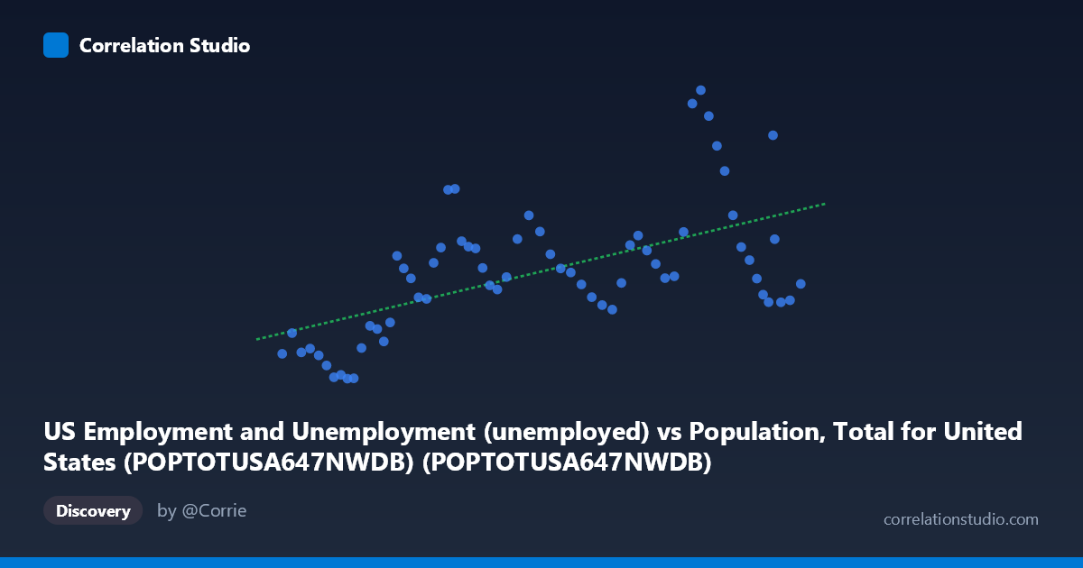
US Employment and Unemployment (unemployed) vs Population, Total for United States (POPTOTUSA647NWDB) (POPTOTUSA647NWDB)
- Pearson correlation (r)
- 0.5759
- Spearman correlation
- 0.5537
- p-value
- 0.000001
- Sample size (n)
- 65
- 95% confidence interval
- 0.3862 to 0.7188
- Granger causality
- None
- Granger optimal lag
- 10
AI analysis
Scatterplot Analysis: US Population vs. Unemployment
Overview of the Relationship
The scatterplot reveals a moderate positive correlation between total US population (X-axis) and the number of unemployed persons (Y-axis) over the period 1960–2024. As population grows from approximately 181 million to 340 million, unemployment counts show a general upward trend, though with considerable scatter around the regression line (y = 3.23×10⁻⁵x − 1,128). This relationship is intuitive on its face — a larger labor force naturally contains more people who may be unemployed at any given time — but the dispersion of points suggests that population size alone is a poor standalone predictor of unemployment levels.
Correlation Strength and Statistical Significance
The Pearson correlation of r = 0.576 indicates a moderate positive relationship, but the more informative metric is r² = 0.332, meaning that US population size explains only about 33% of the variance in unemployment counts. Roughly two-thirds of unemployment variation is driven by factors entirely outside population dynamics. The 95% confidence interval for r of [0.386, 0.719] is relatively wide, reflecting meaningful uncertainty in the true population-level effect, though the p-value of 5.19×10⁻⁷ confirms the correlation is highly unlikely to be a chance finding given n = 65. Critically, Granger causality tests show no significant predictive directionality in either direction (X→Y: F = 0.745, p = 0.678; Y→X: F = 1.581, p = 0.155), meaning that knowing population size does not help forecast future unemployment, and vice versa. This fundamentally undermines any causal interpretation of the correlation.
Notable Patterns and Outliers
Several data points deviate dramatically from the regression line and deserve attention. A cluster of high-unemployment outliers appears in the upper-middle region of the chart — notably points near populations of ~310–332 million with unemployment values of 12,500–14,825 (thousands), which almost certainly correspond to the 2008–2010 Great Recession and the 2020 COVID-19 pandemic shock. These events produced unemployment spikes far beyond what population growth would predict. Conversely, observations at lower population ranges (180–210 million, roughly the 1960s–1970s) cluster tightly with relatively low unemployment values. There is also a visible fan-shaped spread at higher X values, suggesting increasing variance (heteroscedasticity) as population grows — the range of unemployment outcomes widens substantially in recent decades.
Confounding Factors and Caveats
The most significant caveat is that this correlation almost certainly reflects shared time trends rather than a direct structural relationship. Both variables increase over time — population through natural demographic growth, and unemployment counts through labor force expansion — making spurious correlation through common trending a serious concern. The unemployment rate (not count) would be a far more meaningful metric, as it normalizes for population size and would likely show a much weaker or even negligible correlation. Additionally, business cycle effects, monetary policy, technological disruption, globalization, and policy interventions (stimulus programs, unemployment insurance expansions) are major drivers of unemployment that are entirely confounded within this bivariate framework. The wide confidence interval and lack of Granger causality reinforce that this is a descriptive association, not a mechanistic relationship.
Actionable Insights and Further Investigation
Given these limitations, several analytical extensions are recommended. First, replace raw unemployment counts with the unemployment rate to remove the mechanical population-scaling effect and test whether any genuine relationship persists. Second, detrend both series (e.g., using first differences or HP filtering) to isolate cyclical variation from secular trends before computing correlations. Third, incorporate multivariate regression with GDP growth, interest rates, and labor force participation rates as covariates to properly attribute unemployment variance. Fourth, segment the analysis by economic regime (expansion vs. recession periods) to examine whether the correlation differs structurally across business cycles. Finally, consider testing nonlinear models given the visible heteroscedasticity, as the relationship may not be adequately captured by the linear regression applied here.
X dataset: Population, Total for United States (POPTOTUSA647NWDB)
Y dataset: US Employment and Unemployment
Part of experiment: Yearly - Population, Total for United States (POPTOTUSA647NWDB) vs US Employment and Unemployment