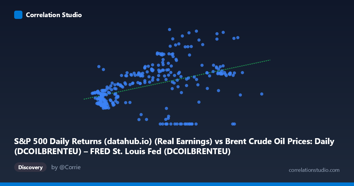
S&P 500 Daily Returns (datahub.io) (Real Earnings) vs Brent Crude Oil Prices: Daily (DCOILBRENTEU) – FRED St. Louis Fed (DCOILBRENTEU)
- Pearson correlation (r)
- 0.4304
- Spearman correlation
- 0.4629
- p-value
- 0
- Sample size (n)
- 297
- 95% confidence interval
- 0.3329 to 0.5188
- Granger causality
- None
- Granger optimal lag
- 3
AI analysis
Brent Crude Oil Prices vs. S&P 500 Real Earnings: Correlation Analysis
Overall Relationship
The scatterplot reveals a modest positive relationship between S&P 500 real earnings (X-axis) and Brent crude oil prices (Y-axis), with the linear regression equation y = 0.627x + 54.923 suggesting that higher real earnings are associated with somewhat higher oil prices. However, the relationship is far from clean — the cloud of points is visibly diffuse, with substantial vertical scatter at nearly every level of X. This wide dispersion immediately signals that real earnings alone explain only a fraction of oil price variation, and that multiple other forces are clearly at work. The broad X range (roughly 10 to 141) and Y range (0 to 217) underscore how dramatically both variables have moved across the nearly four decades of coverage (1987–2026).
Correlation Strength, Statistical Significance, and Causality
The Pearson correlation of r = 0.4304 indicates a weak-to-moderate positive association, but the more telling figure is r² = 0.1853 — meaning real earnings account for only 18.5% of the variance in Brent crude prices, leaving roughly 81.5% explained by other factors entirely. The 95% confidence interval [0.3329, 0.5188] is reasonably narrow given N = 1,865, confirming the correlation is reliably positive but not impressively strong. The p-value of 7.99×10⁻¹⁵ is overwhelmingly significant, but this is largely a function of the very large population size; statistical significance here should not be mistaken for practical or economic significance. Critically, the Granger causality test finds no significant directional predictive relationship in either direction at the optimal 3-period lag (X→Y: F = 2.63, p = 0.050; Y→X: F = 0.47, p = 0.70). The X→Y result sits precisely on the conventional 0.05 threshold — tantalisingly close but not crossing it — while Y→X is clearly non-significant. This means neither variable reliably predicts the other in a temporal sense, and the observed correlation is more likely driven by shared macroeconomic trends than by any direct causal mechanism.
Notable Patterns, Clusters, and Outliers
Several features stand out in the sample points. There is a cluster of low-X, low-to-moderate-Y observations (X < 30, Y in the 40–90 range), likely corresponding to the pre-2000 era when both earnings and oil prices were comparatively subdued. At higher X values (X 70), points spread dramatically in Y — some reaching 177–209 (e.g., 84.51, 209.69; 81.61, 177.43; 83.68, 177.76), while others collapse to near zero (73.63, 0.00; 84.82, 0.00; 86.92, 0.00; 67.09, 0.00). These zero-Y outliers at moderate-to-high X values are particularly striking and likely represent specific crisis periods where oil prices crashed (e.g., 2020 COVID demand collapse, 1998 Asian financial crisis) even while earnings remained relatively robust, or they may reflect data anomalies. The presence of points like (115.55, 115.12) and (113.34, 111.39) at high X with only moderate Y further illustrates that high earnings do not reliably drive high oil prices. There is also a faint suggestion of non-linearity or heteroscedasticity — variance in Y appears to increase with X — which violates a key assumption of simple linear regression.
Confounding Factors and Caveats
Interpreting this correlation requires significant caution. Both variables are heavily influenced by global macroeconomic cycles — during expansion phases, corporate earnings rise and energy demand pushes oil prices up, creating a spurious co-movement that reflects the business cycle rather than any direct link. Geopolitical shocks (Gulf Wars, OPEC supply decisions, Russia-Ukraine conflict) move oil prices independently of earnings entirely. The axis labeling appears swapped relative to what might be economically intuitive — oil prices are on the Y-axis despite being labeled as an X-dataset, which may reflect the analytical framing chosen but risks confusion. Additionally, combining daily oil price data with monthly earnings data introduces temporal aggregation mismatches that can distort correlation estimates. The long time span (1987–2026) means the relationship may be structurally non-stationary; a correlation computed across commodity supercycles and multiple recessions may mask entirely different regime-specific relationships.
Actionable Insights and Further Investigation
Given the weak explained variance and absent Granger causality, real earnings should not be used as a standalone predictor of oil prices in any practical forecasting model. Several next steps would strengthen understanding: (1) Regime-specific analysis — segmenting the data by decade or economic cycle (expansion vs. recession) to test whether the correlation strengthens in particular periods; (2) Multivariate modeling — incorporating USD strength, global industrial production, OPEC output, and inventory levels, which are far stronger oil price determinants; (3) Cointegration testing — checking whether the two series share a long-run equilibrium relationship despite lacking short-term Granger causality; (4) Addressing the zero-Y anomalies — investigating whether the zero oil price observations are genuine (negative futures prices in April 2020?) or data errors, as they materially distort the regression; and (5) Nonlinear or quantile regression to capture the evident heteroscedasticity and potentially reveal threshold effects at extreme earnings levels.
X dataset: Brent Crude Oil Prices: Daily (DCOILBRENTEU) – FRED St. Louis Fed
Y dataset: S&P 500 Daily Returns (datahub.io)
Part of experiment: Daily - Brent Crude Oil Prices: Daily (DCOILBRENTEU) – FRED St. Louis Fed vs S&P 500 Daily Returns (datahub.io)