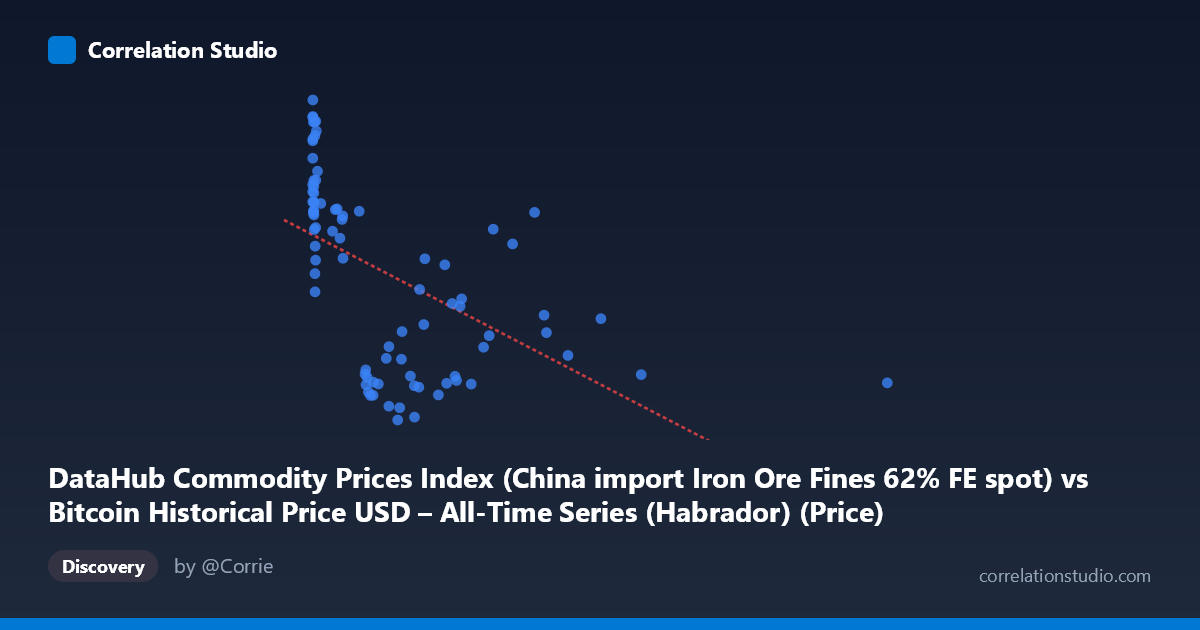
DataHub Commodity Prices Index (China import Iron Ore Fines 62% FE spot) vs Bitcoin Historical Price USD – All-Time Series (Habrador) (Price)
- Pearson correlation (r)
- -0.5301
- Spearman correlation
- -0.7025
- p-value
- 0
- Sample size (n)
- 83
- 95% confidence interval
- -0.6693 to -0.355
- Granger causality
- None
- Granger optimal lag
- 10
AI analysis
Analysis: Iron Ore Price Index vs. Bitcoin Price (2010–2017)
1. What the Visualization Reveals
The scatterplot displays a downward-sloping but noisy relationship between the iron ore commodity price index (X-axis) and Bitcoin's historical USD price (Y-axis). Most data points cluster in the lower-left region (X < 300, Y between 40-140), representing the early Bitcoin era when both prices were relatively low and iron ore trading was concentrated in a modest range. A smaller number of high-X outliers (X 700, extending to 2452) show generally lower Y-values, pulling the trendline downward and driving the negative correlation.
2. Strength, Direction, and Statistical Confidence
The Pearson correlation of r = -0.53 indicates a moderate negative linear relationship, but R² = 0.281 reveals that only about 28% of the variance in Bitcoin price is explained by the iron ore index — leaving 72% unexplained by this single variable. The 95% confidence interval [-0.669, -0.355] is reasonably tight and entirely negative, and the p-value (2.55e-07) is highly significant, confirming this negative association is not due to chance in this sample. However, statistical significance should not be conflated with practical predictive power given the low R².
Critically, the Granger causality tests show no significant predictive direction in either direction (X→Y: p=0.674; Y→X: p=0.485). This means neither variable reliably "leads" the other in time — the correlation is likely contemporaneous/coincidental rather than causal, probably reflecting two independent trends (Bitcoin's early exponential growth phase and iron ore's separate price cycle) that happened to move in opposite directions over this specific historical window rather than any genuine economic linkage.
3. Notable Patterns and Non-linear Features
The data is heavily right-skewed on the X-axis (mean 321, but stdev 405, max 2452), with most points bunched below X=300 and a long tail of sparse high-X outliers. This skew likely distorts the linear fit. The note that Spearman ρ exceeds Pearson r strongly suggests the true relationship is non-linear — possibly logarithmic or curvilinear, where Bitcoin price drops steeply as the index rises from very low values, then flattens out. This is typical of commodity/asset data with power-law or exponential characteristics, common in early Bitcoin price history where values grew from near-zero.
4. Confounding Factors and Caveats
The most significant caveat is that this is a spurious or confounded correlation driven by time, not a direct economic relationship. Bitcoin's price in 2010-2017 was governed by adoption cycles, exchange listings, and speculative bubbles (e.g., the 2013 and 2017 rallies) — entirely unrelated to global iron ore/steel demand dynamics tied to China's construction and manufacturing sector. Since both series are time-ordered and non-stationary (Bitcoin trended upward over time; iron ore had its own cycles independent of Bitcoin), the negative correlation may simply reflect their divergent trends over the same calendar period — a classic case of "correlation without causation" via a shared time index. The small sample size (n=83 paired matches from N=449 possible observations) also limits robustness.
5. Actionable Insights and Further Investigation
Given the lack of Granger causality and the likely spurious nature of this correlation, this relationship should not be used for predictive trading or economic modeling linking iron ore and Bitcoin. Recommended next steps: (1) detrend both series (e.g., using differencing or year-over-year % change) and re-test correlation on stationary data to check if the relationship persists or vanishes; (2) test non-linear fits (log-log or polynomial) given the Spearman/Pearson divergence; (3) investigate whether both variables are driven by a common latent factor (e.g., USD strength, global risk sentiment, or Chinese economic growth) rather than each other; (4) increase the sample size/time overlap to test robustness of the CI.
X dataset: Bitcoin Historical Price USD – All-Time Series (Habrador)
Y dataset: DataHub Commodity Prices Index
Part of experiment: Bitcoin - Bitcoin Historical Price USD – All-Time Series (Habrador) vs DataHub Commodity Prices Index