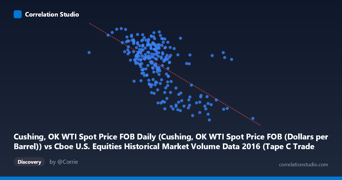
Cushing, OK WTI Spot Price FOB Daily (Cushing, OK WTI Spot Price FOB (Dollars per Barrel)) vs Cboe U.S. Equities Historical Market Volume Data 2016 (Tape C Trade Count)
- Pearson correlation (r)
- -0.6178
- Spearman correlation
- -0.5358
- p-value
- 0
- Sample size (n)
- 252
- 95% confidence interval
- -0.6888 to -0.5351
- Granger causality
- None
- Granger optimal lag
- 1
- Time coverage
- 2016-01-04 to 2016-12-30
- Recomputed on refreshed data
- 2026-10-22 (r was -0.6178)
AI analysis
Analysis: WTI Crude Oil Spot Price vs. Cboe Tape C Trade Count (2016)
Relationship Overview The scatterplot reveals a moderate negative relationship between WTI crude oil spot prices (X-axis, in dollars per barrel) and Cboe Tape C trade counts (Y-axis) across 252 trading days in 2016. As oil prices increase, equity trade counts on Tape C tend to decline, and the linear regression equation (y = −2.85×10⁻⁵x + 63.61) confirms this inverse slope. The relationship is visually apparent but far from deterministic — there is substantial scatter around the regression line, suggesting meaningful variance remains unexplained by price alone.
Correlation Strength and Statistical Significance The Pearson correlation of r = −0.618 indicates a moderate-to-strong negative association, and the p-value of essentially zero confirms this is highly unlikely to be a chance finding given the sample. However, the R² of 0.382 is the critical framing statistic: WTI spot prices explain only ~38% of the variance in Tape C trade counts, meaning roughly 62% of variation is driven by other factors. The 95% confidence interval of [−0.689, −0.535] is reassuringly tight and doesn't approach zero, reinforcing genuine signal. Despite this statistical robustness, the Granger causality tests reveal no significant temporal predictive direction in either direction (X→Y: F=0.694, p=0.406; Y→X: F=0.949, p=0.331). This is a crucial caveat: while the variables co-move contemporaneously, neither reliably leads the other at a one-period lag, suggesting the correlation reflects shared exposure to common drivers rather than a causal pipeline.
Notable Patterns, Clusters, and Outliers Several structural features stand out in the data. There is a distinct cluster of high trade-count observations (Y ≈ 45–52) concentrated in the X range of roughly 500,000–750,000, forming a relatively dense core. Below this cluster, a sparse lower tail of observations with X values exceeding ~850,000–1,000,000 shows markedly lower trade counts (Y ≈ 27–34), pulling the regression slope downward — sample points like (1,023,027; 29.55), (990,202; 33.21), and (849,071; 31.62) are conspicuous high-leverage outliers. The relationship also appears potentially non-linear: the dense mid-range cluster shows relatively flat variation in Y, while the steep drop occurs primarily at the high end of X. This suggests a possible threshold or regime effect rather than a clean linear decline throughout.
Confounding Factors and Caveats Several important caveats apply. First, the axis labels appear to be swapped in the dataset metadata — the X-axis is described as coming from the Cboe volume dataset while the Y-axis is attributed to the WTI price dataset, which is likely a metadata labeling artifact and should be verified before drawing firm conclusions. Second, 2016 was a structurally unusual year for oil markets: prices recovered from multi-year lows (~$26–28/barrel in February 2016) to ~$54 by year-end, meaning trending behavior could be inflating the correlation spuriously (both series following time trends simultaneously). Third, Tape C specifically covers NYSE Arca-listed securities, which skews toward ETFs and energy-sector products — making energy-price sensitivity more pronounced here than in broader market volume measures. Granger non-causality at lag-1 further suggests any relationship may operate at longer lags or through intermediary market sentiment channels.
Actionable Insights and Further Investigation Given these findings, several follow-up analyses are warranted. Detrending both series (e.g., first-differencing or removing the 2016 price recovery trend) would test whether the correlation survives once shared time trends are removed — if it collapses, the relationship is largely spurious. Testing Granger causality at longer lags (2–5 periods) could reveal delayed transmission effects not captured at lag-1. Investigating volatility (e.g., VIX or oil price daily returns) as a mediating variable is promising, since high oil-price environments in 2016 may correlate with low volatility periods that independently suppress trade counts. Finally, segmenting the analysis by quarter would clarify whether the correlation is driven by the early-2016 low-price/high-activity regime versus the late-2016 recovery, which would have significant implications for practical interpretation in trading or risk modeling contexts.
X dataset: Cboe U.S. Equities Historical Market Volume Data 2016
Y dataset: Cushing, OK WTI Spot Price FOB Daily
Part of experiment: Daily - Cboe U.S. Equities Historical Market Volume Data 2016 vs Cushing, OK WTI Spot Price FOB Daily