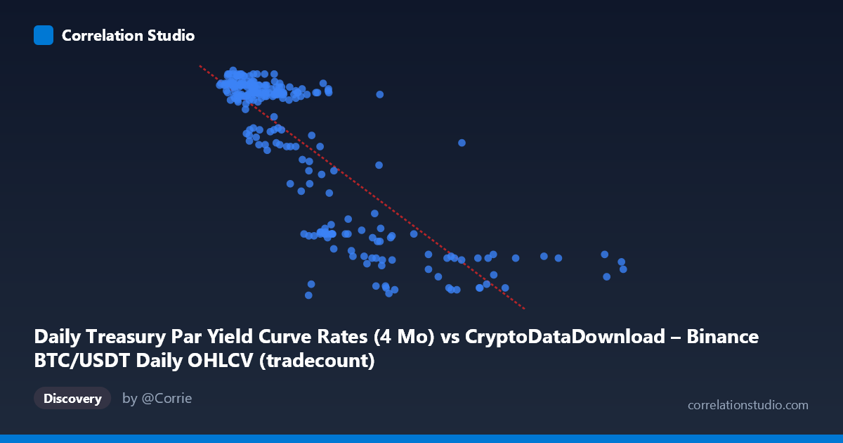
Daily Treasury Par Yield Curve Rates (4 Mo) vs CryptoDataDownload – Binance BTC/USDT Daily OHLCV (tradecount)
- Pearson correlation (r)
- -0.8197
- Spearman correlation
- -0.7966
- p-value
- 0
- Sample size (n)
- 250
- 95% confidence interval
- -0.8566 to -0.7744
- Granger causality
- None
- Granger optimal lag
- 1
- Time coverage
- 2024-01-02 to 2024-12-31
AI analysis
Analysis of Treasury Yield vs. BTC/USDT Metric Relationship
Note on labeling: The axis metadata appears mismatched (X is labeled as Treasury yield data but shows values in the millions, consistent with tradecount; Y ranges 4.3–5.5, consistent with a yield percentage). This analysis proceeds based on the actual data behavior — X as a high-magnitude count-like variable (likely tradecount) and Y as a bounded percentage-like variable (likely the 4-month yield) — while noting this ambiguity should be resolved before drawing firm conclusions.
1. Relationship Overview The scatterplot reveals a clear negative, moderately-strong nonlinear relationship. As X increases from ~1M to ~12M, Y declines steadily from ~5.5 to ~4.3. The relationship is not perfectly linear — it resembles a decelerating curve (steep drop-off at low X values, flattening at high X), though the linear fit still captures the dominant trend reasonably well.
2. Strength, Direction, and Statistical Confidence The Pearson correlation of r = -0.82 indicates a strong negative association, with r² = 0.672 meaning roughly 67% of the variance in Y is explained by X (linearly) — a substantial but not complete relationship, leaving ~33% driven by other factors or nonlinear dynamics. The 95% CI [-0.857, -0.774] is tight and entirely negative, and the p-value ≈ 0 confirms this correlation is highly statistically significant and not due to chance, given n=250.
However, the Granger causality tests show no significant predictive direction: X→Y is marginal (F=3.69, p=0.056, just missing conventional significance) while Y→X shows no signal at all (p=0.85). This means that despite the strong contemporaneous correlation, neither variable reliably predicts the other's future values at a 1-period lag. This is a critical distinction: correlation ≠ Granger-causal predictability. The relationship may be driven by a shared underlying trend or external factor rather than one variable mechanically leading the other.
3. Patterns and Clusters Two visually distinct clusters emerge: - A dense cluster at low X (1M–4M) with Y consistently high (5.2–5.5) — this comprises the majority of points (~80%) - A sparser tail at high X (5M–12M) with Y dropping to 4.3–4.5
The transition zone (X ≈ 3M–5M) shows more scatter and variability (Y ranging 4.5–5.4), suggesting this is where the relationship is least stable — potentially a regime-change zone. The high-X outliers (8M–12M range) pull the tail of the trend downward and have outsized leverage on the linear fit.
4. Confounding Factors and Caveats - Metadata mismatch: The axis labels appear swapped or misattributed between the two datasets (Treasury yields vs. BTC tradecount), which raises concerns about data integrity — this should be verified before publishing conclusions. - Time-series autocorrelation: Both series likely trend smoothly over the year (2024-01-02 to 2024-12-31), so the strong r may partly reflect shared temporal drift (e.g., both declining/rising over the year) rather than a direct causal link — classic spurious correlation risk in time series. - Nonlinearity: The visible curve shape suggests a linear r² may understate or mischaracterize the true relationship; a log or power transform of X might fit better. - Sparse high-X data: Few points above X=6M mean the tail behavior is less statistically robust and more sensitive to outliers.
5. Suggested Next Steps - Verify column/axis labeling to ensure Treasury yield and tradecount data haven't been swapped. - Detrend or difference both series (e.g., day-over-day changes) and re-run correlation/Granger tests to check if the relationship holds beyond shared trend — this is essential given the Granger results already hint that the levels relationship may not be causal. - Test nonlinear fits (log, exponential, or piecewise) given the visible curvature. - Segment analysis: separately examine the dense low-X cluster vs. the high-X tail, as they may represent different market regimes (e.g., different volatility or rate environments). - Extend lag structure in Granger tests (beyond lag 1) to check for delayed effects, since the X→Y result was close to significance and longer lags might reveal a true predictive relationship.
X dataset: CryptoDataDownload – Binance BTC/USDT Daily OHLCV
Y dataset: Daily Treasury Par Yield Curve Rates
Part of experiment: Bitcoin - CryptoDataDownload – Binance BTC/USDT Daily OHLCV vs Daily Treasury Par Yield Curve Rates