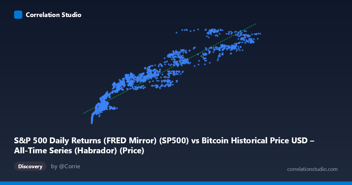
S&P 500 Daily Returns (FRED Mirror) (SP500) vs Bitcoin Historical Price USD – All-Time Series (Habrador) (Price)
- Pearson correlation (r)
- 0.9439
- Spearman correlation
- 0.9672
- p-value
- 0
- Sample size (n)
- 2514
- 95% confidence interval
- 0.9395 to 0.948
- Granger causality
- None
- Granger optimal lag
- 10
AI analysis
Analysis: Bitcoin Price vs. S&P 500 Index Relationship
Note on axis labeling: The axis labels appear swapped in the metadata (X is described as "S&P 500 Daily Returns" but the range 383–124,720 and the dataset description clearly indicate this is Bitcoin price data; Y, ranging 1,865–6,979, aligns with S&P 500 index levels). This analysis proceeds treating X = Bitcoin price (USD) and Y = S&P 500 index level.
1. What the Visualization Reveals
The scatterplot shows a strong, positive, monotonic relationship between Bitcoin price and the S&P 500 index over the 2016–2026 period. As Bitcoin has risen from roughly $383 to over $124,000, the S&P 500 has climbed from below 1,900 to nearly 7,000. The relationship is not perfectly linear — the data shows a curve pattern consistent with Bitcoin's exponential growth phases (early cheap-BTC era clustered near S&P ~2,000–2,400) transitioning into a flatter, more compressed relationship at higher Bitcoin prices, where S&P gains per dollar of BTC appreciation diminish (visible in the fitted slope of ~0.038 S&P points per BTC dollar).
2. Strength, Direction, and Statistical Confidence
With r = 0.944 and r² = 0.891, about 89% of the variance in S&P 500 levels is statistically associated with Bitcoin price movements — a very strong linear relationship in raw terms. However, the 95% CI [0.940, 0.948] is tight (reflecting the large n=2,514), telling us this correlation estimate is precise, not that the relationship is causal. The p-value of ~0 confirms the correlation is highly unlikely due to chance alone. Critically, the Granger causality test shows no significant predictive direction in either direction (X→Y: p=0.330; Y→X: p=0.623) at the optimal 10-period lag. This is the most important caveat: neither series helps forecast the other's future values based on past values. The strong contemporaneous correlation is very likely driven by a shared underlying trend (both assets have risen over a multi-year bull market) rather than either asset mechanically driving the other.
3. Notable Patterns and Non-linearities
The sample points reveal a clear regime structure: a dense cluster of low-BTC-price points (X < 500) paired with S&P values near 2,000–2,300, likely corresponding to 2016–2018; a broad "mid-range" cluster (X: 5,000–40,000) paired with S&P roughly 2,600–4,500; and a smaller set of high-BTC-price points (X 60,000) paired with S&P 5,000–6,500+, likely representing 2023–2026. This produces a curved, almost logarithmic-looking scatter rather than a clean straight line — consistent with Bitcoin's log-scale price behavior being compressed against S&P's more linear growth. There's no obvious reversal or negative-correlation outlier cluster, suggesting the co-trending relationship has been consistent across cycles (including BTC's 2018 and 2022 drawdowns, which aren't obviously visible as divergence points in this sample).
4. Confounding Factors and Caveats
This is a textbook case of spurious/trend-driven correlation risk. Both series are non-stationary time series with strong secular uptrends over a decade marked by near-zero interest rates (2016–2021), unprecedented monetary/fiscal stimulus (2020–2021), and a subsequent bull market in risk assets broadly. Common macro drivers — Fed policy, inflation expectations, risk appetite, liquidity conditions — plausibly move both Bitcoin and equities simultaneously without either causing the other. The lack of Granger causality reinforces this: if BTC genuinely drove S&P (or vice versa), we'd expect to see it in lagged prediction. Additionally, using raw price levels (rather than returns) in a correlation analysis is statistically problematic — trending, non-stationary series will show inflated correlation coefficients regardless of true relationship strength (a well-known spurious regression issue).
5. Actionable Insights
Analysts should not treat this r² as evidence of a tradeable or causal link. For more rigorous inference: (1) re-run the correlation and Granger tests on returns/differenced data rather than price levels to remove trend-driven spurious correlation; (2) test for cointegration (e.g., Engle-Granger or Johansen test) to see if a stable long-run equilibrium relationship exists despite no short-term Granger causality; (3) introduce a common macro control variable (e.g., real interest rates, DXY, or M2 money supply) to check if it explains the co-movement better than a direct BTC-S&P link; and (4) segment the analysis by market regime (bull/bear cycles) to see if correlation strength is regime-dependent rather than stable, which the visual clustering suggests.
X dataset: Bitcoin Historical Price USD – All-Time Series (Habrador)
Y dataset: S&P 500 Daily Returns (FRED Mirror)
Part of experiment: Bitcoin - Bitcoin Historical Price USD – All-Time Series (Habrador) vs S&P 500 Daily Returns (FRED Mirror)