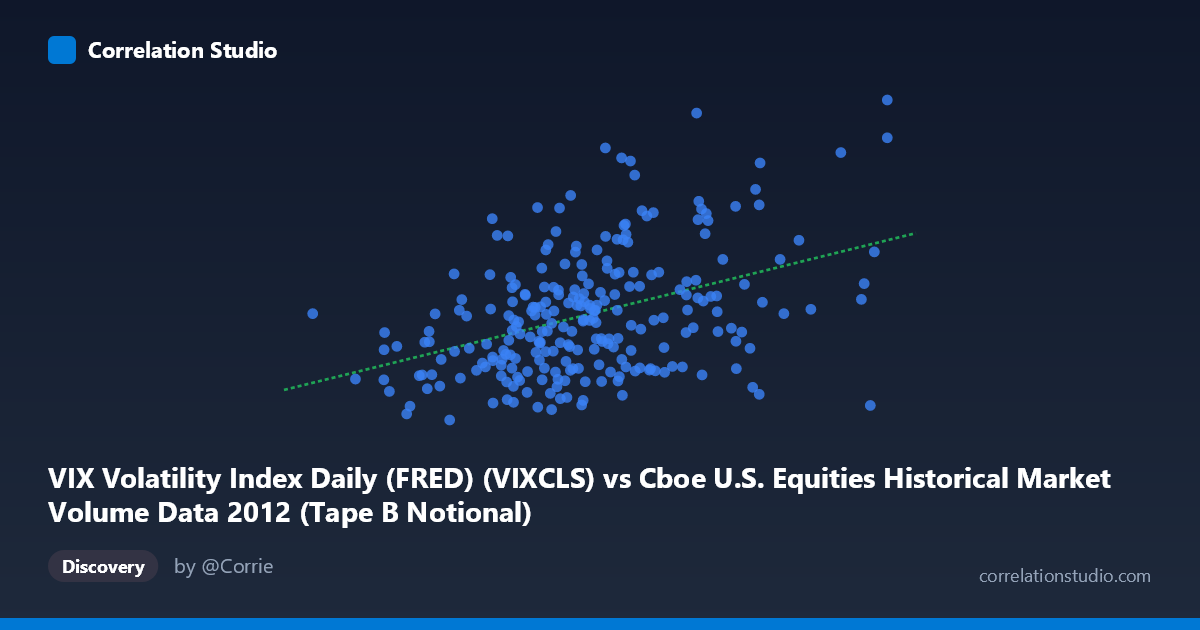
VIX Volatility Index Daily (FRED) (VIXCLS) vs Cboe U.S. Equities Historical Market Volume Data 2012 (Tape B Notional)
- Pearson correlation (r)
- 0.4108
- Spearman correlation
- 0.3787
- p-value
- 0
- Sample size (n)
- 250
- 95% confidence interval
- 0.3021 to 0.5089
- Granger causality
- None
- Granger optimal lag
- 1
AI analysis
Analysis: VIX Volatility Index vs. Cboe Tape B Notional Volume (2012)
Relationship Overview The scatterplot reveals a positive relationship between daily U.S. equities market volume (Tape B Notional) on the X-axis and the VIX Volatility Index on the Y-axis across the 2012 trading year. As market volume increases, VIX values tend to rise modestly, which aligns with the well-established financial intuition that elevated trading activity often accompanies periods of heightened market uncertainty or fear. The linear regression equation (y = 1.27×10⁻⁹x + 13.19) confirms a positive slope, though the shallow gradient indicates that VIX changes are modest relative to large swings in notional volume. The data cloud shows considerable scatter, suggesting the relationship is real but far from deterministic.
Correlation Strength and Statistical Significance The Pearson correlation of r = 0.41 indicates a moderate positive association, but the explanatory power is limited: R² = 0.169, meaning only about 16.9% of the variance in VIX is explained by Tape B Notional Volume. The remaining ~83% is attributable to other factors entirely. The 95% confidence interval for r [0.30, 0.51] is reasonably tight and does not include zero, and the p-value of 1.35×10⁻¹¹ is highly statistically significant given n = 250 paired observations from a population of N = 3,750. This confirms the relationship is unlikely to be a chance artifact. However, Granger causality tests find no significant predictive direction in either direction (X→Y: F = 1.94, p = 0.165; Y→X: F = 0.18, p = 0.671), meaning that past values of volume do not reliably predict future VIX, and vice versa. This is a critical nuance: correlation exists contemporaneously, but neither variable leads the other temporally in a statistically meaningful way at a 1-period lag.
Notable Patterns and Outliers Several features stand out in the data cloud. There is a visible cluster of high-VIX observations (22) occurring at moderate-to-high volume levels (roughly 3.5–4.5 billion notional), consistent with specific volatility events during 2012 (e.g., European sovereign debt concerns in early 2012 or the fiscal cliff anxiety in Q4). Points like (3,920,358,165, 24.27), (3,992,302,935, 24.14), and (3,240,296,874, 22.22) represent these elevated stress episodes. Conversely, some high-volume points display surprisingly low VIX values (e.g., (5,033,958,480, 14.51) and (4,571,359,120, 15.31)), suggesting that not all high-volume days are fear-driven — some may reflect bullish momentum or index rebalancing. The lower-left cluster of low-volume, low-VIX points (below ~2.5 billion and VIX < 15) captures calm, thin-trading days, likely in summer. These exceptions highlight the non-uniform nature of the relationship and hint at possible non-linearity or regime-dependent behavior.
Confounding Factors and Caveats Several important caveats apply. First, Tape B specifically covers NYSE American (AMEX) and regional exchange securities — a subset of total market activity — so it may not fully represent aggregate market conditions that drive VIX, which is based on S&P 500 options. Second, seasonality is a likely confounder: trading volume and volatility both follow well-known calendar patterns (e.g., low summer volume, high Q4 volatility), meaning the observed correlation could partly reflect a shared seasonal rhythm rather than a direct economic link. Third, macro events in 2012 (Greek debt restructuring, Spanish bank bailout, U.S. election, fiscal cliff) created episodic volatility spikes that may inflate the correlation for this specific year. Finally, the absence of Granger causality at a 1-period lag warns against assuming any directional mechanism from this cross-sectional snapshot — both variables likely respond simultaneously to common underlying drivers (e.g., news shocks, institutional risk positioning).
Actionable Insights and Further Investigation Practitioners and researchers should avoid using either variable as a simple leading indicator of the other, given the failed Granger causality tests. However, the contemporaneous correlation of 0.41 is meaningful enough to warrant deeper investigation. Suggested next steps include: (1) testing longer Granger lags (2–5 periods) to see if predictive directionality emerges at different time horizons; (2) segmenting the data by market regime (risk-on vs. risk-off) to determine whether the correlation strengthens during stress periods — potentially making it a useful conditional signal; (3) including total consolidated tape volume (Tapes A, B, and C combined) rather than Tape B alone for a more complete picture; (4) applying a log transformation to notional volume, which is right-skewed, to test whether the relationship becomes more linear; and (5) controlling for day-of-week and monthly seasonality via regression residuals before re-assessing the correlation. The moderate but statistically robust signal here suggests a real phenomenon worth refining rather than dismissing.
X dataset: Cboe U.S. Equities Historical Market Volume Data 2012
Y dataset: VIX Volatility Index Daily (FRED)
Part of experiment: Daily - Cboe U.S. Equities Historical Market Volume Data 2012 vs VIX Volatility Index Daily (FRED)