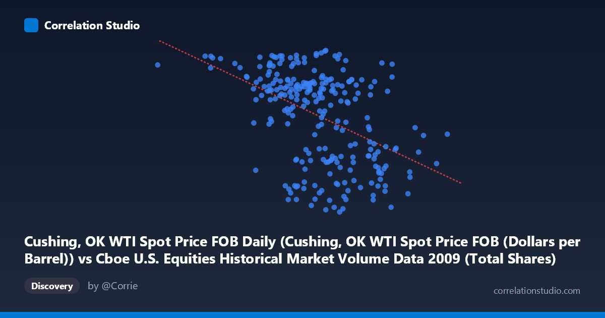
Cushing, OK WTI Spot Price FOB Daily (Cushing, OK WTI Spot Price FOB (Dollars per Barrel)) vs Cboe U.S. Equities Historical Market Volume Data 2009 (Total Shares)
- Pearson correlation (r)
- -0.4531
- Spearman correlation
- -0.4389
- p-value
- 0
- Sample size (n)
- 252
- 95% confidence interval
- -0.5461 to -0.3491
- Granger causality
- None
- Granger optimal lag
- 1
AI analysis
WTI Crude Oil Price vs. U.S. Equity Market Trading Volume (2009)
Relationship Overview
The scatterplot reveals a moderate negative relationship between WTI crude oil spot prices (X-axis) and U.S. equity market total shares traded (Y-axis) across 252 paired daily observations in 2009. As oil prices rise, equity trading volume tends to decline, and vice versa. This inverse pattern is visually apparent in the data cloud, though with considerable scatter around the regression line (y = -3.90×10⁻⁸x + 91.60). The relationship reflects the broader macroeconomic dynamics of 2009, a year defined by the tail end of the financial crisis, a dramatic oil price recovery from near $30/barrel lows in early 2009 to ~$80/barrel by year-end, and an equity market that was simultaneously volatile and gradually recovering — conditions that likely drove these two series in opposing directions for much of the year.
Correlation Strength and Statistical Significance
The Pearson correlation of r = -0.453 indicates a moderate negative association, and the r² of 0.205 means that approximately 20.5% of the variance in equity trading volume is statistically explained by WTI oil prices. While statistically meaningful, this also means that nearly 80% of the variance in trading volume is driven by other factors not captured in this bivariate relationship. The 95% confidence interval for r spans [-0.546, -0.349], which is reasonably tight and entirely negative, reinforcing that the inverse direction of the relationship is robust and not an artifact of sampling. The p-value of 3.66×10⁻¹⁴ is extraordinarily small, providing overwhelming evidence against the null hypothesis of no correlation — this is a statistically real signal in the data. However, the Granger causality tests tell a more cautious story: neither direction (X→Y nor Y→X) yields significant predictive power at the optimal lag of 1 period (F = 0.61, p = 0.43 for oil→volume; F = 0.12, p = 0.73 for volume→oil). This means that knowing yesterday's oil price does not meaningfully improve our ability to predict today's trading volume, and vice versa — the correlation is contemporaneous and associative rather than temporally predictive.
Notable Patterns, Clusters, and Outliers
Several structural features stand out in the sample points. There is a visible cluster of high trading volume observations (Y 70) concentrated at lower oil price levels (roughly $40–$65/barrel, corresponding to early 2009 during peak crisis volatility), while lower trading volumes tend to appear at higher oil prices (above $90–$100/barrel, corresponding to the second half of 2009 as markets stabilized). This is consistent with the regression line's negative slope. There are notable outliers in both directions: the point near (192,269,942, 76.83) represents an extreme low oil price with high volume, likely from early January 2009 during severe market stress, while points near (1,212,524,830, 56.67) and (1,073,811,434, 39.35) suggest that at very high oil prices, volumes can vary widely. The spread in Y values at any given X level is substantial (spanning 30–45 percentage-point ranges), confirming the weak-to-moderate nature of the relationship and hinting at possible non-linear or regime-dependent dynamics — for instance, the relationship may behave differently during periods of acute financial stress versus calmer trending markets.
Confounding Factors and Interpretive Caveats
Several important caveats apply. First, 2009 is a highly atypical year — it captured both the depths of the global financial crisis (Q1) and a powerful recovery rally (Q2–Q4), meaning both oil prices and equity volumes were simultaneously responding to a common third driver: macroeconomic risk sentiment and investor fear. This creates a classic spurious correlation via confounding: both variables were likely being driven by the VIX, credit spreads, and broader deleveraging dynamics rather than by a direct causal mechanism linking oil to equity trading activity. Second, the units and scales merit attention — WTI prices are in dollars per barrel while total shares represents aggregate U.S. equity market volume, making the direct economic mechanism unclear without further mediation analysis. Third, the linear regression model may be oversimplifying what could be a piecewise or threshold relationship: the dynamics in a crisis environment (oil below $50) may be fundamentally different from a recovery environment (oil above $70). Finally, the N=3,232 population vs. n=252 sample suggests this analysis covers sampled data, and any temporal autocorrelation in daily financial time series can inflate the apparent precision of standard correlation tests.
Actionable Insights and Further Investigation
Despite the lack of Granger causality, this correlation is informative and warrants deeper investigation along several dimensions. First, a regime-segmented analysis — splitting the data at the market bottom (approximately March 2009) — could reveal whether the negative correlation is stronger or weaker during crisis vs. recovery phases, which would have implications for risk modeling. Second, introducing VIX or credit spread data as a control variable in a multivariate regression would help isolate whether the oil-volume relationship persists after accounting for the dominant fear/risk-appetite driver. Third, extending this analysis across multiple years (not just 2009) would test whether the negative correlation is a structural feature of these markets or a crisis-specific artifact — if it disappears in non-crisis years, it should not be used for general inference. Fourth, given the absence of Granger causality at a 1-day lag, testing longer lags (5–10 days) or using weekly aggregations might uncover delayed transmission mechanisms. Finally, practitioners in algorithmic trading or macro-factor modeling could use this relationship as a confirming signal rather than a standalone predictor — pairing oil price direction with other macro signals when building equity volume forecasts for liquidity planning or execution strategy.
X dataset: Cboe U.S. Equities Historical Market Volume Data 2009
Y dataset: Cushing, OK WTI Spot Price FOB Daily
Part of experiment: Daily - Cboe U.S. Equities Historical Market Volume Data 2009 vs Cushing, OK WTI Spot Price FOB Daily