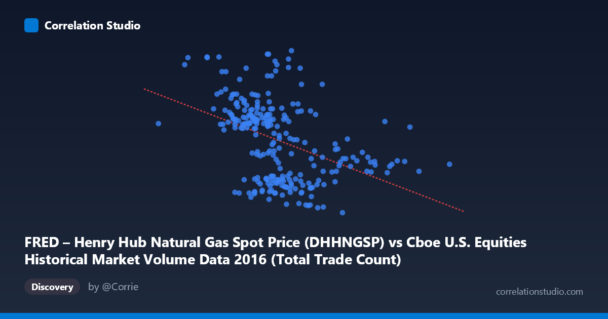
FRED – Henry Hub Natural Gas Spot Price (DHHNGSP) vs Cboe U.S. Equities Historical Market Volume Data 2016 (Total Trade Count)
- Pearson correlation (r)
- -0.4196
- Spearman correlation
- -0.4624
- p-value
- 0
- Sample size (n)
- 252
- 95% confidence interval
- -0.5164 to -0.3123
- Granger causality
- None
- Granger optimal lag
- 1
AI analysis
Analysis: Henry Hub Natural Gas Spot Price vs. Cboe U.S. Equities Total Trade Count (2016)
Relationship Overview The scatterplot reveals a modest negative relationship between Henry Hub Natural Gas Spot prices (X-axis, measured in $/MMBtu) and Cboe U.S. Equities Total Trade Count (Y-axis) across 252 trading days in 2016. The linear regression equation (y = -4.45278E⁻⁰⁷x + 3.596) confirms this downward slope: as natural gas prices increase, equity trade counts tend to decrease slightly. However, the scatter is considerable, and the relationship is far from deterministic. Visually, the data cloud is broadly dispersed, with no tight clustering around the regression line, suggesting that many other forces are driving trade count variation throughout the year.
Correlation Strength, Direction, and Statistical Significance The Pearson correlation of r = -0.420 indicates a weak-to-moderate negative association. More informatively, r² = 0.176, meaning natural gas prices explain only about 17.6% of the variance in equity trade counts — leaving roughly 82% of variation unexplained by this single predictor. The 95% confidence interval of [-0.516, -0.312] is reasonably tight and excludes zero, and the p-value of 3.6×10⁻¹² confirms the correlation is highly statistically significant, effectively ruling out chance as an explanation given n = 252. That said, statistical significance here is partly a function of the large population (N = 3,622) and the precision of the estimate rather than evidence of a strong or practically meaningful effect. Critically, the Granger causality tests find no significant predictive directionality in either direction (X→Y: F = 0.831, p = 0.363; Y→X: F = 0.335, p = 0.563), meaning natural gas prices do not temporally predict trade counts at the following period, and vice versa. This strongly argues against any direct causal or leading-indicator relationship between these two variables.
Notable Patterns, Clusters, and Outliers Examining the sample points, several features stand out. There is a notable concentration of data points with X values between roughly 1.9M and 2.7M (the core trading volume range), within which Y values span nearly the full range from ~1.77 to ~3.56 $/MMBtu — illustrating the weak explanatory power visually. A few apparent outliers are worth noting: the point near (1,722,715, 3.50) represents an unusually low trade count paired with a relatively high gas price, and (2,538,868, 3.56) shows a high gas price at moderate trade volume. At the upper end of the X-axis, points near 3.3M–4.5M trade counts cluster at lower gas prices (around $2.15–$2.26), which is consistent with the negative slope but represents a relatively sparse region of observations. There is also no obvious non-linear curvature visible; the relationship, while weak, appears reasonably linear across its range.
Confounding Factors and Caveats The most important caveat is that this correlation almost certainly reflects coincidental co-movement driven by shared seasonal or calendar effects rather than any fundamental economic linkage. Both natural gas prices and equity market volumes have strong seasonal patterns in 2016: gas prices were historically low early in the year and rose through winter months, while equity trade volumes may have followed distinct patterns tied to earnings seasons, volatility events (e.g., Brexit, U.S. elections), and end-of-year rebalancing. This creates a spurious correlation through time as a common confounder. Additionally, the unit mismatch is notable — X represents market microstructure activity (number of trades) while Y represents a commodity spot price — and there is no plausible direct mechanism by which one would cause the other. The absence of Granger causality corroborates this. Selection of 2016 as a single year also limits generalizability, as this was a particularly unusual year for both energy markets and financial markets.
Actionable Insights and Further Investigation Given the weak explanatory power and absence of Granger causality, this correlation should not be used for trading or forecasting purposes in its current form. However, the finding is not entirely without value. Analysts could investigate whether the correlation is driven by specific sub-periods — for example, periods of energy market stress (Q1 2016 gas price lows) coinciding with elevated market volatility and trade counts. A logical next step would be to partial out seasonality from both series and re-test the correlation on the residuals; if the correlation disappears, it confirms a seasonal confound. It would also be worthwhile to extend the analysis across multiple years to assess whether the r = -0.42 finding in 2016 is stable or an artifact of that year's unique conditions. Finally, incorporating additional variables — such as the VIX (equity volatility index), energy sector equity volumes specifically, or broader macroeconomic indicators — into a multivariate framework would help determine whether any residual relationship between these two series survives proper controls.
X dataset: Cboe U.S. Equities Historical Market Volume Data 2016
Y dataset: FRED – Henry Hub Natural Gas Spot Price
Part of experiment: Daily - Cboe U.S. Equities Historical Market Volume Data 2016 vs FRED – Henry Hub Natural Gas Spot Price