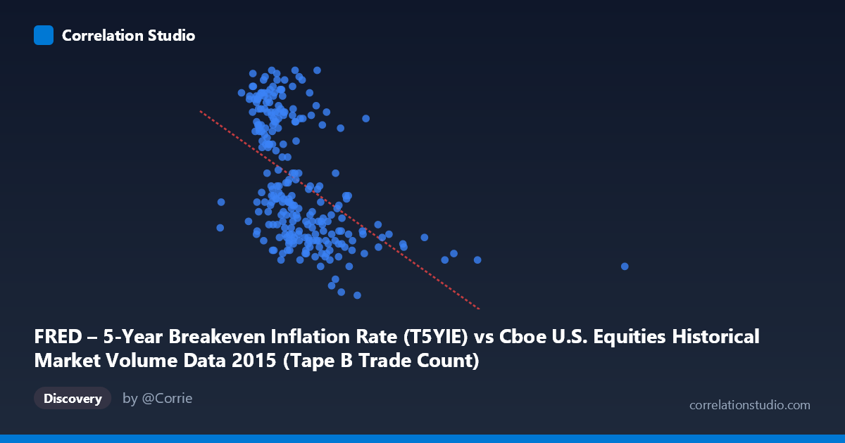
FRED – 5-Year Breakeven Inflation Rate (T5YIE) vs Cboe U.S. Equities Historical Market Volume Data 2015 (Tape B Trade Count)
- Pearson correlation (r)
- -0.4971
- Spearman correlation
- -0.5851
- p-value
- 0
- Sample size (n)
- 250
- 95% confidence interval
- -0.5851 to -0.3976
- Granger causality
- None
- Granger optimal lag
- 1
AI analysis
Scatterplot Analysis: 5-Year Breakeven Inflation Rate vs. Cboe Tape B Trade Count (2015)
Relationship Overview
The scatterplot reveals a negative relationship between the Cboe U.S. Equities Tape B Trade Count (X-axis) and the 5-Year Breakeven Inflation Rate (Y-axis) across 2015 trading days. As daily equity trade volume increases, the breakeven inflation rate tends to be lower, and conversely, lower-volume days cluster toward higher inflation expectations. The linear regression equation (y = -1.01085E-06x + 1.68019) reflects this inverse slope, with the relationship most visually evident in the bulk of observations concentrated between roughly 130,000–500,000 trade counts and inflation rates spanning 1.10–1.72. The scatter is considerable, indicating this is a noisy, imperfect relationship rather than a clean linear signal.
Correlation Strength and Statistical Framing
The Pearson correlation of r = -0.497 indicates a moderate negative association, but the explanatory power deserves careful framing: r² = 0.247 means only 24.7% of the variance in the inflation breakeven rate is explained by trade count, leaving roughly three-quarters of variation unexplained by this relationship alone. The 95% confidence interval of [-0.585, -0.398] is entirely negative and does not cross zero, confirming the direction is statistically reliable across the sampled range. The p-value of effectively zero (given N = 3,302) confirms this correlation is highly unlikely to be a chance artifact at the population level. However, Granger causality tests find no significant predictive directionality in either direction — neither X→Y (F = 0.321, p = 0.572) nor Y→X (F = 1.015, p = 0.315) — meaning that knowing today's trade volume does not meaningfully improve forecasts of tomorrow's inflation expectations, and vice versa. The relationship appears contemporaneous and associative rather than temporally predictive.
Patterns, Clusters, and Outliers
Several structural features stand out in the data. The bulk of observations form a dense cluster between 130,000–450,000 trade counts and 1.10–1.70 inflation rates, where the negative trend is most visible. There is a notable upper-left cluster — days with relatively low trade volume (150,000–280,000) but high inflation rates (1.55–1.72) — which appears to pull the regression slope strongly. Conversely, a lower-right grouping of higher-volume days (350,000–500,000) is associated predominantly with lower inflation rates (1.10–1.30). A small number of extreme outliers are visible at very high trade counts (notably one observation near 1,014,000 and another around 692,000), which sit at low inflation levels (~1.10–1.13) and likely exert disproportionate leverage on the regression slope. These extreme volume days may reflect specific market events (e.g., heightened volatility episodes in August 2015) that simultaneously drove volume spikes and suppressed inflation expectations.
Confounding Factors and Interpretive Caveats
The axes in this dataset are notably swapped from their natural roles — the X-axis carries the inflation rate data label while the Y-axis carries the trade count label, which is worth flagging as a potential source of interpretive confusion when reading the regression. More substantively, 2015 was a year of significant macro events — Federal Reserve rate normalization anticipation, the August 2015 Chinese equity market shock, and commodity price declines — all of which could simultaneously depress inflation expectations and spike trading volume, creating a spurious or confounded correlation rather than a genuine structural link. Breakeven inflation rates are themselves a financial market construct and may co-move with equity market stress indicators for reasons unrelated to actual inflation dynamics. Additionally, Tape B specifically covers NYSE American and regional exchanges, so trade count here is not a complete proxy for total U.S. equity market activity, limiting generalizability.
Actionable Insights and Further Investigation
Given the moderate but unexplained 75% residual variance and the absence of Granger causality, this correlation is best treated as a contextual market-regime indicator rather than a predictive tool. Analysts should investigate whether the relationship holds across other years or is specific to 2015's unique macro environment — a multi-year panel analysis would clarify this. It would also be valuable to control for VIX or credit spreads, as market stress likely mediates both volume and inflation expectations simultaneously. Decomposing the data by sub-period (pre/post August 2015 correction) could reveal whether the correlation is driven entirely by a handful of crisis days. Finally, expanding beyond Tape B to aggregate U.S. equity volume and pairing with other inflation measures (e.g., 10-year breakeven, CPI surprises) would help determine whether this inverse relationship reflects a genuine risk-off/inflation expectations mechanism or is largely an artifact of the 2015 sample period.
X dataset: Cboe U.S. Equities Historical Market Volume Data 2015
Y dataset: FRED – 5-Year Breakeven Inflation Rate
Part of experiment: Daily - Cboe U.S. Equities Historical Market Volume Data 2015 vs FRED – 5-Year Breakeven Inflation Rate