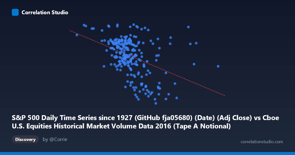
S&P 500 Daily Time Series since 1927 (GitHub fja05680) (Date) (Adj Close) vs Cboe U.S. Equities Historical Market Volume Data 2016 (Tape A Notional)

Pearson correlation (r): -0.4172
Spearman correlation: -0.428
p-value: 0
Sample size (n): 252
95% confidence interval: -0.5143 to -0.3096
Granger causality: None
Granger optimal lag: 4

AI analysis

Scatterplot Analysis: S&P 500 Adjusted Close vs. Tape A Notional Volume (2016)

Relationship Overview The scatterplot reveals a moderate negative relationship between S&P 500 adjusted closing prices (X-axis) and Cboe Tape A notional trading volume (Y-axis) across 252 trading days in 2016. The linear regression equation (y = -2.39×10⁻⁸x + 2309.17) indicates that as the S&P 500 price level rises, Tape A notional volume tends to decline. Visually, the data points form a downward-sloping cloud without tight clustering around the regression line, suggesting the relationship exists but is far from deterministic. The wide spread of Y values at any given X reinforces that price level alone is a poor predictor of notional volume on any single day.

Correlation Strength and Statistical Significance The Pearson correlation of r = -0.4172 reflects a moderate negative association, but the explanatory power is modest: r² = 0.1741 means only 17.4% of the variance in Tape A notional volume is explained by the S&P 500 price level, leaving roughly 82.6% attributable to other factors. The 95% confidence interval of [-0.5143, -0.3096] is meaningfully negative throughout — it does not cross zero — and the p-value of 4.93×10⁻¹² confirms the relationship is highly statistically significant and extremely unlikely to be a chance artifact given n = 252 paired observations from a population of 3,622. However, statistical significance here is partly a function of sample size; the practical magnitude of the effect remains limited. Critically, Granger causality tests show no significant predictive direction in either direction (X→Y: F = 0.41, p = 0.80; Y→X: F = 1.08, p = 0.37), meaning neither variable reliably leads or predicts the other across the tested lag structure of 4 periods. The correlation is contemporaneous at best, not temporally predictive.

Notable Patterns, Clusters, and Outliers Several features stand out in the data. There is a visible cluster of points in the upper-left quadrant — lower S&P 500 price levels (roughly 7–8 billion on the X scale, consistent with earlier 2016 dates) paired with higher notional volumes (above ~2,150) — which drives much of the negative slope. Conversely, points at higher X values (later in 2016, post-election rally) tend to show lower notional volume, though with substantial scatter. A handful of apparent outliers deserve attention: one point near X ≈ 6.78B shows an exceptionally high Y (~2,265), and another cluster near X ≈ 10.5–10.8B shows unusually low Y values (~1,869–1,883), which are well below the regression line and may correspond to specific market events such as the post-Brexit volatility period or pre-election quiet. The point at approximately (9,581M, 2,262) also sits far above the trend. These outliers exert leverage on the regression slope and may distort the overall correlation estimate.

Confounding Factors and Caveats Several important caveats apply to interpreting this correlation. First, the X-axis is labeled as a date column (adjusted close from S&P 500 data) being plotted numerically, meaning the X values likely represent Unix timestamps or serial date numbers, not prices directly — the range of ~3.7B to ~17.6B is inconsistent with S&P 500 price history and strongly suggests raw date encoding. This means the negative correlation may primarily reflect a time trend: early 2016 saw market volatility and elevated volume, while later 2016 (especially post-November election rally) saw rising index levels with declining Tape A volume as trading may have shifted across venues or calmed. Second, notional volume is price-dependent by construction — higher prices mean the same number of shares generates higher notional value, which could theoretically work against a negative correlation, making the observed negative result more substantively interesting. Third, venue fragmentation and TRF reporting changes during 2016 could independently shift Tape A notional figures irrespective of price levels.

Actionable Insights and Further Investigation Given the time-trend confound, the most immediate recommendation is to re-examine this relationship with time explicitly controlled — either by detrending both series, using returns/changes rather than levels, or including date as a covariate in a multivariate regression. Researchers should also decompose Tape A notional volume by market event periods (e.g., Brexit in June, U.S. election in November) to test whether outliers represent structural breaks or regime changes rather than continuous relationships. Since Granger causality was non-significant, trading strategies based on one series predicting the other would not be supported by this data; however, testing at shorter intraday lags or with alternative lag selection criteria could yield different results. Finally, incorporating total market volume, VIX (volatility index), and venue market share data as additional variables would likely improve explanatory power well beyond the current 17.4% and help isolate whether this correlation reflects genuine economic linkage or is primarily a shared trend artifact.

X dataset: Cboe U.S. Equities Historical Market Volume Data 2016

Y dataset: S&P 500 Daily Time Series since 1927 (GitHub fja05680) (Date)

Part of experiment: Daily - Cboe U.S. Equities Historical Market Volume Data 2016 vs S&P 500 Daily Time Series since 1927 (GitHub fja05680) (Date)