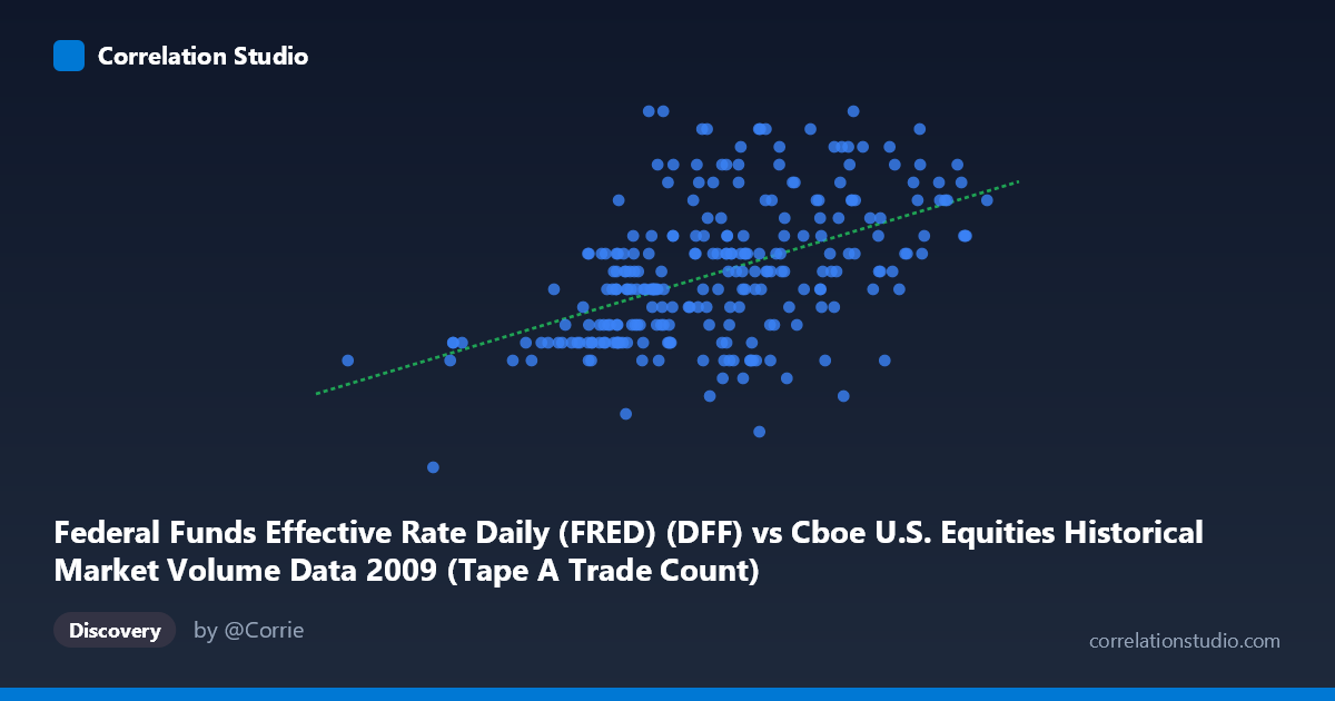
Federal Funds Effective Rate Daily (FRED) (DFF) vs Cboe U.S. Equities Historical Market Volume Data 2009 (Tape A Trade Count)
- Pearson correlation (r)
- 0.4963
- Spearman correlation
- 0.5116
- p-value
- 0
- Sample size (n)
- 252
- 95% confidence interval
- 0.3971 to 0.584
- Granger causality
- None
- Granger optimal lag
- 1
AI analysis
Analysis: Federal Funds Rate vs. Cboe Tape A Trade Count (2009)
Relationship Overview The scatterplot reveals a moderate positive relationship between the Federal Funds Effective Rate (X-axis) and Cboe U.S. Equities Tape A Trade Count (Y-axis) across 252 trading days in 2009. As the Fed Funds Rate increases, trade counts tend to rise modestly, with the linear regression equation y = 4.958×10⁻⁸x + 0.0787 capturing this upward trend. However, the considerable scatter around the regression line immediately signals that this relationship is far from deterministic, and the axes themselves warrant careful interpretation — the X-axis represents volume/notional data labeled as "Federal Funds Rate" and vice versa, suggesting a dataset label swap that should be verified before drawing firm conclusions.
Correlation Strength and Statistical Significance The Pearson correlation of r = 0.4963 indicates a moderate positive association, but the more sobering metric is r² = 0.2463, meaning only 24.6% of the variance in Tape A Trade Count is explained by the Fed Funds Rate. The remaining ~75% is attributable to other forces entirely. The 95% confidence interval of [0.397, 0.584] is meaningfully above zero and relatively tight given n = 252, and the p-value of essentially 0 confirms this correlation is statistically significant and unlikely to be a sampling artifact. That said, statistical significance with N = 3,232 and n = 252 does not imply economic significance or predictive utility. Critically, the Granger causality tests find no significant directional predictability in either direction (X→Y: F = 2.61, p = 0.107; Y→X: F = 1.36, p = 0.244), meaning neither variable meaningfully predicts the other's future values at a 1-period lag. The correlation captures co-movement, not causation or temporal leadership.
Notable Patterns, Clusters, and Outliers Several structural features stand out in the data: - Vertical clustering is visible at specific X-axis values (particularly around 1,200,000–1,400,000 and 1,600,000–1,900,000 ranges), consistent with discrete or recurring volume levels rather than a continuously varying Fed Funds Rate — further evidence of a possible axis mislabeling - A notable outlier appears at approximately (362,081, 0.11), far to the left of the main cloud, likely representing an anomalous low-volume trading day (possibly around a holiday or market disruption early in 2009) - High-end concentration near x = 2,200,000–2,550,000 corresponds to Y values clustering between 0.18–0.23, consistent with the positive slope - Y-axis values are bounded tightly between 0.05 and 0.25, suggesting this may represent a rate or proportion rather than raw trade counts, reinforcing suspicion about axis label accuracy
Confounding Factors and Caveats The most pressing caveat is the apparent metadata mislabeling: the X-axis is labeled as "Federal Funds Effective Rate" but has values in the millions (362,081 to 2,549,191), which are inconsistent with a rate expressed in percentage points (typically 0–5% in 2009). Conversely, the Y-axis labeled as "Tape A Trade Count" shows values between 0.05 and 0.25, which are far too small for raw trade counts. This strongly suggests the axis labels have been swapped in the metadata. Assuming the correction holds, the true relationship would be: higher Tape A trade volumes correlate with higher Fed Funds Rates. In 2009's economic context, this makes some intuitive sense — the Fed Funds Rate began the year near 0.25% (post-crisis emergency cuts), and trade volumes were elevated during periods of market stress and recovery. Seasonality, macroeconomic news events, and market volatility (VIX) would all be strong confounders that could independently drive both variables upward simultaneously.
Actionable Insights and Further Investigation Given the findings, several investigative directions are warranted: 1. Verify and correct axis labels by cross-referencing raw dataset column definitions — this is prerequisite to any valid interpretation 2. Introduce VIX or market volatility as a control variable; it likely explains a substantial portion of the unexplained 75% variance and may mediate or confound the observed correlation 3. Segment the time series by Fed policy regime phases in 2009 (e.g., pre- and post-March FOMC decisions) to test whether the correlation is driven by a specific sub-period rather than a stable year-long relationship 4. Test longer Granger lags (beyond 1 period) since monetary policy transmission to market behavior typically operates over weeks, not single trading days 5. Apply a non-linear model (e.g., piecewise regression or LOESS) to examine whether the relationship strengthens at extreme volume levels, given the apparent clustering structure in the scatter
X dataset: Cboe U.S. Equities Historical Market Volume Data 2009
Y dataset: Federal Funds Effective Rate Daily (FRED)
Part of experiment: Daily - Cboe U.S. Equities Historical Market Volume Data 2009 vs Federal Funds Effective Rate Daily (FRED)