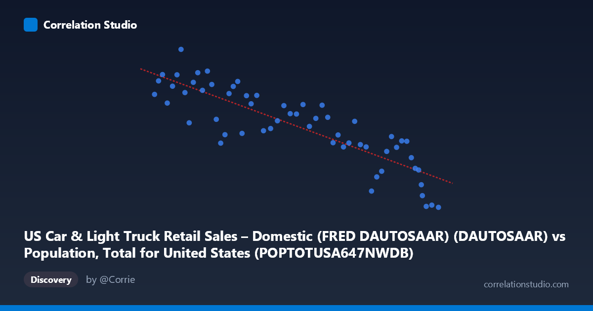
US Car & Light Truck Retail Sales – Domestic (FRED DAUTOSAAR) (DAUTOSAAR) vs Population, Total for United States (POPTOTUSA647NWDB) (POPTOTUSA647NWDB)
- Pearson correlation (r)
- -0.8556
- Spearman correlation
- -0.8688
- p-value
- 0
- Sample size (n)
- 58
- 95% confidence interval
- -0.9123 to -0.7668
- Granger causality
- None
- Granger optimal lag
- 1
- Time coverage
- 1967-01-01 to 2024-01-01
- Recomputed on refreshed data
- 2026-10-20 (r was -0.8556)
AI analysis
Analysis: US Population vs. Domestic Auto Sales
Relationship Overview The scatterplot reveals a strong negative relationship between US total population (X-axis) and domestic car & light truck retail sales (Y-axis), which is immediately counterintuitive — as the US population has grown over the 1967–2024 period, domestic auto sales have trended downward. The linear regression equation (y = -3.76×10⁻⁸x + 16.36) confirms this inverse trajectory, with sales declining roughly 0.038 units (in millions SAAR) for every additional person in the US population. Since population grows monotonically over time, this relationship is essentially a proxy for a long-run secular decline in domestic auto sales relative to what might be expected from a growing consumer base.
Correlation Strength and Statistical Robustness The Pearson correlation of r = -0.856 is strong, and the R² of 0.732 means that approximately 73.2% of the variance in domestic auto sales is statistically explained by variation in population — a substantial share for a single predictor. The 95% confidence interval of [-0.912, -0.767] is notably tight and sits entirely in negative territory, leaving no ambiguity about the direction of the association. The p-value of effectively zero confirms this is not a chance finding. However, the Granger causality results undercut any causal interpretation: neither direction (X→Y: F=1.28, p=0.263; Y→X: F=0.017, p=0.898) achieves significance, meaning population does not temporally predict auto sales, nor vice versa. This strongly signals that both variables are being driven by a shared underlying factor — time — rather than one causing the other.
Patterns, Clusters, and Notable Features The data naturally clusters into two broad regimes. Points in the lower-left region (population ~198M–245M, roughly 1967–1990) generally show higher domestic sales values (7–10 million SAAR), while points in the upper-right region (population ~280M–340M, roughly 2000–2024) cluster at lower sales figures (2–7 million SAAR). Several outliers merit attention: the extreme low-sales observations near 2.07–2.18 (population ~336M–340M) likely correspond to the COVID-19 disruption (2020–2021) and associated supply chain crises that devastated auto production. Conversely, the high-sales point near 10.14 (population ~212M) may reflect a mid-1970s or early-1980s peak demand period. The relationship appears broadly linear but with notable scatter in the middle range (~250M–295M population), suggesting structural breaks or cyclical volatility that a simple linear model cannot fully capture.
Confounding Factors and Caveats The most critical caveat is spurious correlation via shared time trend: both population and domestic auto sales are indexed to the same years (1967–2024), and population grows nearly monotonically, making it a near-perfect stand-in for a time index. The true drivers of declining domestic auto sales are more plausibly: (1) rising import penetration from Japanese and European automakers eroding domestic market share; (2) demand saturation and shifting consumer preferences toward SUVs and trucks (which may be partially captured here); (3) economic cycles — recessions in 1973, 1981, 2008–09, and 2020 all suppressed sales; and (4) fuel price shocks. None of these are controlled for, meaning the population-sales correlation is almost certainly confounded by the passage of time and structural industry change rather than reflecting a true demographic mechanism.
Actionable Insights and Further Investigation Analysts should detrend both series (e.g., using first differences or per-capita normalization) before drawing any structural conclusions — expressing domestic sales per capita or per driving-age adult would immediately neutralize the spurious time-trend component and likely reveal a more nuanced picture. It would be worthwhile to decompose the decline by separating domestic vs. import market share data, which would test whether total light vehicle sales (domestic + foreign) actually track population more naturally. Additionally, incorporating GDP, fuel prices, credit conditions, and import share as covariates in a multivariate model would clarify how much of the variance attributed to population is actually attributable to these economic drivers. Finally, structural break testing (e.g., Chow test around 1980 or 2008) could formally identify whether the relationship has shifted across different automotive eras, improving forecasting precision for industry planning purposes.
X dataset: Population, Total for United States (POPTOTUSA647NWDB)
Y dataset: US Car & Light Truck Retail Sales – Domestic (FRED DAUTOSAAR)
Part of experiment: Yearly - Population, Total for United States (POPTOTUSA647NWDB) vs US Car & Light Truck Retail Sales – Domestic (FRED DAUTOSAAR)