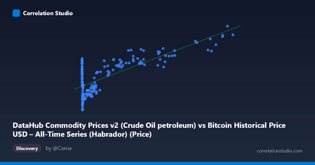
DataHub Commodity Prices v2 (Crude Oil petroleum) vs Bitcoin Historical Price USD – All-Time Series (Habrador) (Price)
- Pearson correlation (r)
- 0.76
- Spearman correlation
- 0.4787
- p-value
- 0
- Sample size (n)
- 182
- 95% confidence interval
- 0.6909 to 0.8153
- Granger causality
- None
- Granger optimal lag
- 2
- Time coverage
- 2010-08-01 to 2025-09-01
- Recomputed on refreshed data
- 2026-10-24 (r was 0.76)
AI analysis
Analysis: Bitcoin Price vs. Crude Oil Commodity Price
1. Relationship Overview
The scatterplot displays a strongly positive, non-linear relationship between Bitcoin's historical price (X-axis, spanning from fractions of a cent to $113,500) and crude oil commodity prices (Y-axis, ranging $85.78–$238.51). The data shows a classic logarithmic/power-law curve rather than a straight line: at low Bitcoin values (under $1,000), Y values cluster tightly in the $85–$160 range with considerable scatter, while as Bitcoin prices climb into the tens of thousands, Y values rise steadily and more predictably toward the $170–$220 range. This curvature suggests the linear model, while statistically significant, is not the ideal functional form for this data.
2. Strength, Direction, and Statistical Confidence
The correlation coefficient (r = 0.76) indicates a strong positive linear association, with r² = 0.578 meaning Bitcoin's price explains roughly 58% of the variance in the commodity price series — a substantial but incomplete share, leaving 42% attributable to other factors or non-linear dynamics. The 95% confidence interval [0.691, 0.815] is reasonably tight and entirely excludes zero, and the p-value (~0) confirms this correlation is highly unlikely to be due to chance. However, the Granger causality tests are the critical caveat here: neither direction (X→Y: p=0.474; Y→X: p=0.880) shows significant predictive causality at the optimal 2-period lag. This is an important distinction — strong correlation does not imply temporal predictive power. The two series move together contemporaneously (likely both reflecting long-term macro trends or shared time-based drift) but knowing one series' past values does not help forecast the other's future values.
3. Notable Patterns and Outliers
The most striking feature is the extreme heteroskedasticity: variance in Y is much tighter at low X values and widens somewhat at high X values, though the overall trend still tightens into a recognizable curve at the upper end. Several low-X, high-Y outliers stand out (e.g., X=0.92, Y=170.99; X=3.03, Y=172.84; X=6.08, Y=165.00) — these represent Bitcoin's earliest history (2010-2011) when prices were near-zero but commodity prices were already elevated, likely due to unrelated global conditions (e.g., post-2008 recovery, oil price cycles). The high-X tail (X50,000) shows a tighter, more linear-looking cluster, suggesting the relationship may stabilize or that both series simply trended upward together during 2020–2024.
4. Confounding Factors and Caveats
This correlation is very likely spurious or indirect, driven by a shared confound: time itself. Both Bitcoin's price and commodity/oil prices have exhibited long-term secular uptrends over the 2010–2025 window (Bitcoin due to adoption/speculation cycles, oil due to inflation, geopolitical events, and demand growth). Two unrelated time series that both trend upward will show high correlation without any causal mechanism connecting them. The lack of Granger causality in either direction strongly supports this interpretation — there's no evidence Bitcoin prices drive oil prices or vice versa; they're likely both proxies for broader macroeconomic time trends (inflation, USD strength, monetary policy). Additionally, the massive scale disparity in X (0.06 to 113,500) suggests a log transformation of X would likely be more appropriate and could reveal whether the "real" relationship is much weaker (or stronger) once trend components are removed.
5. Recommendations for Further Investigation
Before drawing any economic conclusions, analysts should: (1) detrend both series (e.g., via differencing or removing a fitted trend) and re-examine correlation on returns/changes rather than levels, which typically eliminates spurious time-driven correlations; (2) apply a log-transform on X given its multi-order-of-magnitude range, and test whether a log-linear model fits better than r²=0.578; (3) run a cointegration test to properly assess long-run equilibrium relationships, which is more appropriate than Granger causality for two non-stationary trending series; and (4) explicitly control for a shared time/macro variable (e.g., include a time trend or USD index as a covariate) to determine whether the residual correlation between Bitcoin and oil prices holds any meaningful signal once common trend effects are stripped away.
X dataset: Bitcoin Historical Price USD – All-Time Series (Habrador)
Y dataset: DataHub Commodity Prices v2
Part of experiment: Bitcoin - Bitcoin Historical Price USD – All-Time Series (Habrador) vs DataHub Commodity Prices v2