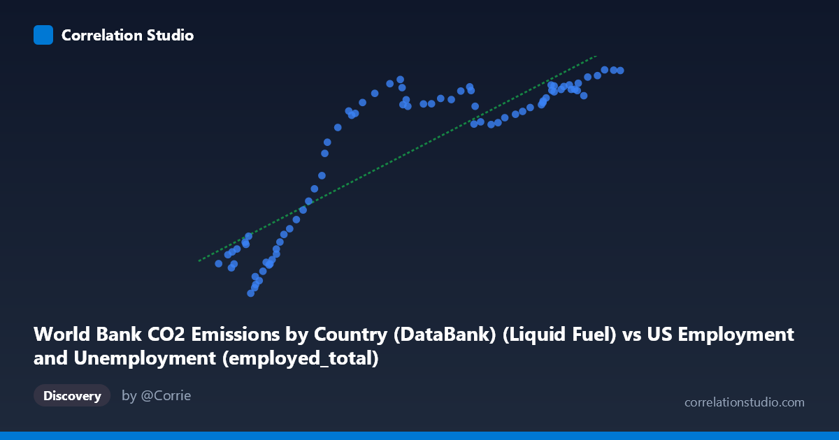
World Bank CO2 Emissions by Country (DataBank) (Liquid Fuel) vs US Employment and Unemployment (employed_total)
- Pearson correlation (r)
- 0.8779
- Spearman correlation
- 0.8754
- p-value
- 0
- Sample size (n)
- 80
- 95% confidence interval
- 0.8155 to 0.9201
- Granger causality
- None
- Granger optimal lag
- 10
AI analysis
Scatterplot Analysis: US Liquid Fuel CO2 Emissions vs. Total US Employment (1941–2020)
1. Overall Relationship
The scatterplot reveals a strong positive association between US liquid fuel CO2 emissions (X-axis) and total US employment (Y-axis) across eight decades of annual observations. As emissions rise from roughly 50,000 to 157,000 units, employed totals climb correspondingly from approximately 2,500 to 13,600 (thousands). The fitted linear regression line (y = 0.09623x − 231.659) tracks the data reasonably well across the mid-range, though the scatter is visibly heterogeneous — tighter clustering at the upper end of the emissions spectrum and noticeably wider dispersion in the lower-to-mid range, suggesting the relationship may not be purely linear throughout.
2. Correlation Strength, Direction, and Temporal Predictive Power
The Pearson correlation of r = 0.8779 indicates a strong positive linear relationship, and the R² of 0.7707 means that approximately 77% of the variance in total employment is statistically explained by variation in liquid fuel emissions within this sample — a substantial proportion, though it also means roughly 23% of variability remains unaccounted for by this single predictor. The 95% confidence interval for r of [0.8155, 0.9201] is relatively narrow and lies entirely above 0.8, confirming that the strength of this association is estimated with good precision and is unlikely to be a sampling artifact. The p-value of effectively 0 (given n = 80) confirms the correlation is highly statistically significant. However, the Granger causality analysis tells a critically different story: neither direction — emissions predicting employment (F = 1.10, p = 0.38) nor employment predicting emissions (F = 0.94, p = 0.51) — reaches statistical significance, even at an optimal lag of 10 periods. This means that despite the strong contemporaneous correlation, neither variable temporally predicts the other in a causal time-series sense. The two variables move together historically, but one does not reliably lead the other.
3. Notable Patterns, Clusters, and Outliers
The data distributes into two visually distinct zones. The lower-left cluster (emissions ~50,000–80,000; employment ~2,500–8,000) corresponds to earlier decades (1940s–1970s), where several data points scatter substantially away from the regression line — most strikingly, a handful of points with low emissions but relatively modest employment figures that sit noticeably below the trend (e.g., the point near (58,918; 2,497), likely a wartime or early postwar year). The upper-right cluster (emissions ~110,000–157,000; employment ~10,000–13,600) representing later decades shows much tighter adherence to the regression line, suggesting the linear model fits the modern era better than the historical one. A moderate "gap" in the middle range (~80,000–110,000 emissions) is also apparent, which may reflect structural shifts in the US economy during transitional decades. There are no extreme leverage outliers that would single-handedly distort the regression, but the lower-left dispersion warrants attention.
4. Confounding Factors and Interpretive Caveats
This correlation almost certainly reflects shared temporal trends rather than a direct mechanistic link between liquid fuel combustion and employment levels. Both variables are strongly driven by a common underlying factor: overall US economic and population growth over time. A growing economy simultaneously demands more energy (hence more liquid fuel emissions) and employs more people — making the correlation largely spurious in a causal sense, which is precisely what the Granger analysis confirms. Additional confounders include: wartime mobilization dynamics in the 1940s, oil price shocks in the 1970s–80s, recessions (2001, 2008–09), the COVID-19 shock of 2020, and structural shifts toward service-sector employment that decoupled energy intensity from job counts in later decades. The dataset mismatch in labeling (the X variable is labeled as from a "US Employment" dataset while representing CO2 data, and vice versa) also warrants careful verification before drawing conclusions. Furthermore, using annual aggregates smooths over cyclical and seasonal dynamics that could reveal very different short-term relationships.
5. Actionable Insights and Further Investigation
Given the strong correlation but absent Granger causality, the most productive next steps would be: (a) Detrending both series (e.g., using first differences or percent changes) to isolate whether a relationship persists beyond shared secular growth trends — this would likely substantially reduce r; (b) Including GDP or population as a covariate to test whether the emissions–employment correlation survives controlling for the primary confound; (c) Segmenting the analysis by era (pre-1970, 1970–2000, post-2000) to test structural stability, given the visible heteroscedasticity; (d) Exploring non-linear specifications (e.g., logarithmic or piecewise regression), particularly for the lower-emission historical period where the linear fit appears weakest; and (e) Repeating Granger testing at shorter lags (1–3 periods) to check whether the null result holds at policy-relevant timescales. The analysis is most useful as a descriptive historical portrait of co-evolving macroeconomic and energy trends rather than as evidence of any actionable directional relationship.
X dataset: US Employment and Unemployment
Y dataset: World Bank CO2 Emissions by Country (DataBank)
Part of experiment: Yearly - US Employment and Unemployment vs World Bank CO2 Emissions by Country (DataBank)