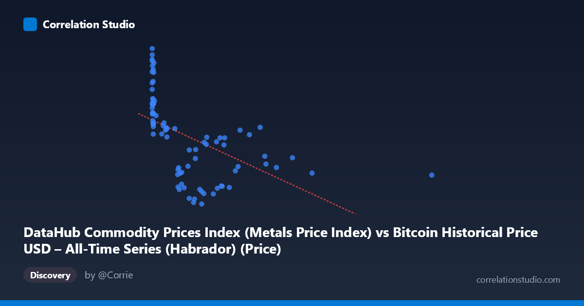
DataHub Commodity Prices Index (Metals Price Index) vs Bitcoin Historical Price USD – All-Time Series (Habrador) (Price)
- Pearson correlation (r)
- -0.5274
- Spearman correlation
- -0.7572
- p-value
- 0
- Sample size (n)
- 83
- 95% confidence interval
- -0.6672 to -0.3517
- Granger causality
- None
- Granger optimal lag
- 3
AI analysis
Analysis: Bitcoin Price vs. Metals Price Index
1. What the Visualization Reveals
The scatterplot shows a moderate negative relationship between the Metals Price Index (X) and Bitcoin's historical USD price (Y), though the label orientation is somewhat unusual—this appears to actually be tracking how Bitcoin's price behaved relative to metals index values over time (2010–2017). The data is heavily clustered at low X-values (under ~250), with a long, sparse tail extending to X=2452.18. This clustering pattern is critical: the vast majority of observations sit in a narrow X-band while a handful of high-leverage points sit far to the right, likely exerting outsized influence on the linear fit.
2. Strength, Direction, and Statistical Confidence
The Pearson correlation (r = -0.5274) indicates a moderate negative linear association, with r² = 0.278 meaning only 27.8% of the variance in Y is explained by X — the majority of variability (72%) is driven by other factors. The 95% CI [-0.667, -0.352] is reasonably tight and excludes zero, and the p-value (3.02E-07) is highly significant, confirming this correlation is not due to chance. However, statistical significance with modest effect size means the relationship is real but not strongly predictive on a point-by-point basis.
The Granger causality results are important: neither variable significantly predicts the other (X→Y p=0.499; Y→X p=0.356). This strongly suggests the correlation is not a causal or lead-lag relationship in time, but more likely reflects a spurious correlation — both series may be independently trending (e.g., both influenced by macroeconomic cycles, USD strength, or simply both trending over the 2010-2017 window) rather than one driving the other.
3. Notable Patterns and Outliers
- Dense low-X cluster (X < 50): Points here show wide Y variation (104–256), indicating high noise/heterogeneity when Bitcoin metric values are low. - Sparse high-X tail (X 700): Points like (2452.18, 132.40), (1402.08, 134.37) are isolated and could disproportionately drag the regression slope negative — classic leverage-point risk. - Non-linearity flagged: Spearman ρ exceeding Pearson r is a signal that a monotonic but non-linear relationship (log, power, or saturating curve) may fit better than the straight line, consistent with the compressed clustering at low X and stretched tail at high X — a hallmark of data needing log-transformation on the X-axis.
4. Confounding Factors and Caveats
- Time confound: Both series span 2010–2017 and may share macro-level trends (dollar strength, global risk sentiment, post-financial-crisis commodity supercycle unwinding) independent of any real interaction. - Small sample, uneven sampling: n=83 paired points from a population of 449 — sampling gaps could bias which portions of each series' cycle are captured. - Heteroscedasticity: Variance in Y is much larger at low X, violating linear regression assumptions and inflating apparent scatter. - Mismatched axis labeling: The dataset descriptions suggest X and Y labels may be swapped or mismatched — this should be verified before drawing economic conclusions.
5. Actionable Insights
- Re-run with log(X) transformation: Given the skewed X distribution and Spearman/Pearson divergence, refit using log or rank-based models to better capture the true monotonic relationship. - Treat correlation as descriptive, not causal: Given the null Granger result, avoid using this relationship for forecasting one series from the other. - Investigate a common driver: Look for a third time-indexed variable (e.g., USD index, global liquidity/interest rates) that could jointly explain trends in both series. - Robustness check: Remove or downweight the high-leverage tail points (X 1000) and re-assess r² to test sensitivity of the correlation to those few observations.
X dataset: Bitcoin Historical Price USD – All-Time Series (Habrador)
Y dataset: DataHub Commodity Prices Index
Part of experiment: Bitcoin - Bitcoin Historical Price USD – All-Time Series (Habrador) vs DataHub Commodity Prices Index