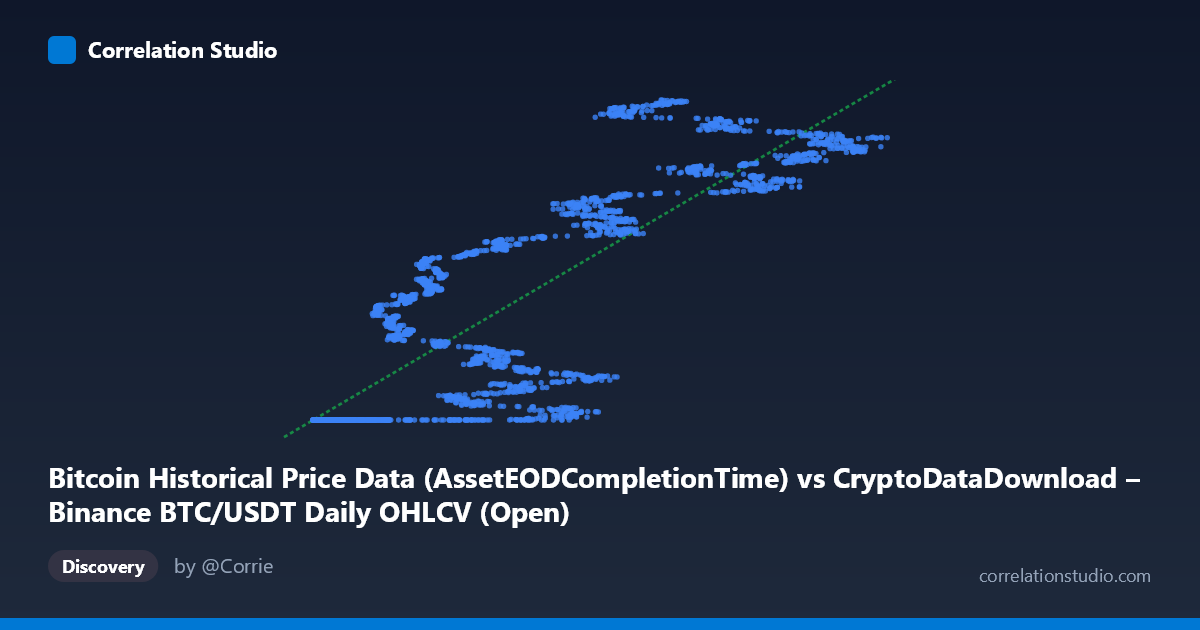
Bitcoin Historical Price Data (AssetEODCompletionTime) vs CryptoDataDownload – Binance BTC/USDT Daily OHLCV (Open)
- Pearson correlation (r)
- 0.8518
- Spearman correlation
- 0.8876
- p-value
- 0
- Sample size (n)
- 3191
- 95% confidence interval
- 0.842 to 0.8611
- Granger causality
- None
- Granger optimal lag
- 10
- Time coverage
- 2017-08-17 to 2026-05-20
AI analysis
Analysis: BTC/USDT AssetEODCompletionTime vs. Open Price
1. What the Visualization Reveals
At face value, this scatterplot appears to compare two variables — but closer inspection of the underlying data reveals that the "X" column (labeled as a completion timestamp) is actually behaving as a proxy for time/price index, not an independent economic variable. The Y-axis (BTC/USDT Open price) is the actual asset price. The sample points show a highly structured, non-random pattern: a large cluster of X-values below ~30,000 are all associated with a nearly constant Y-value (~1,614,337,xxx), while X-values above ~30,000 show Y climbing steadily toward ~1,779,332,997. This is not a typical bivariate scatter — it looks like X is essentially an index or sequence number correlated with the chronological ordering of price observations, with Y being the price itself expressed in a scaled/offset format.
2. Strength, Direction, and Statistical Confidence
The Pearson correlation of r = 0.8518 (r² = 0.7256) indicates a strong positive linear relationship, with X explaining about 72.6% of the variance in Y. The 95% CI [0.8420, 0.8611] is tight, and p ≈ 0 confirms this relationship is not due to chance at this sample size (n = 3,191). Practically, this means that as X increases, Y increases in a highly predictable, near-linear fashion (slope ≈ 1,429.5 per unit X). However, the Granger causality tests show no significant predictive direction in either direction (X→Y: p = 0.33; Y→X: p = 0.15) at 10 lags. This is a critical caveat: a strong contemporaneous correlation does not imply that one variable temporally leads or forecasts the other. This pattern is classic for two series that are both driven by an underlying trend (e.g., calendar time or monotonic price appreciation) rather than a causal feedback relationship.
3. Notable Patterns and Non-linear Features
The sample points reveal a two-regime structure rather than a single linear trend: - A flat "floor" cluster: many X-values between ~3,700 and ~30,000 map to an almost identical Y-value near 1,614,337,xxx (varying only in the last 2-3 digits). This suggests these are early observations where price was pinned near a base/minimum value (possibly BTC's 2018-2019 bear-market lows, scaled). - A rising trend cluster: X-values from ~30,000 to ~124,000 show Y increasing steadily and with more scatter, up to ~1,779,332,997.
This bimodal behavior strongly suggests non-linear, possibly logarithmic or regime-dependent structure — a simple linear r²=0.73 masks the fact that a large subset of the data has near-zero variance in Y while another subset drives most of the correlation. A piecewise or log-linear model would likely fit better than a single linear regression.
4. Confounding Factors and Caveats
- Autocorrelation/non-stationarity: Both series span 2017–2026 and are almost certainly time-ordered; financial price series are non-stationary and trend heavily, which inflates correlation coefficients between any two monotonically trending series (spurious correlation risk). - Scale/unit ambiguity: The X variable, described as a "completion timestamp," and Y being in raw price units with a 1.6-billion offset, suggests a data-formatting artifact (e.g., Unix timestamps or scaled price fields) rather than a meaningful economic relationship. - Structural breaks: The flat-then-rising pattern indicates possible regime shifts (bear market → bull market) that a single correlation/regression coefficient cannot capture. - No causal mechanism: Given the Granger test results, treating this correlation as predictive or causal for trading/forecasting purposes would be inappropriate.
5. Actionable Recommendations
- Clarify variable definitions: Confirm whether X truly represents a timestamp/index and Y a raw or scaled price; if so, this analysis is essentially "price vs. time," which should be modeled with time-series methods (ARIMA, trend decomposition) rather than simple linear correlation. - Segment the data: Split into the flat-price regime (X < 30,000) and rising regime (X ≥ 30,000) and analyze each separately, or apply a log or piecewise model to better capture the true functional form. - Test for stationarity and detrend: Apply differencing or detrending before recomputing correlation to check if the relationship holds beyond shared trend. - Extend Granger analysis: Given no causality was found at 10 lags, test other lag structures or use cross-correlation functions to identify if any lead-lag relationship exists at shorter horizons (e.g., 1-5 periods) relevant to trading strategies.
X dataset: CryptoDataDownload – Binance BTC/USDT Daily OHLCV
Y dataset: Bitcoin Historical Price Data
Part of experiment: Bitcoin - CryptoDataDownload – Binance BTC/USDT Daily OHLCV vs Bitcoin Historical Price Data