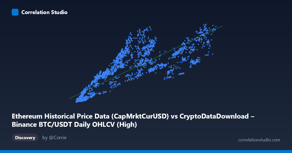
Ethereum Historical Price Data (CapMrktCurUSD) vs CryptoDataDownload – Binance BTC/USDT Daily OHLCV (High)
- Pearson correlation (r)
- 0.8491
- Spearman correlation
- 0.913
- p-value
- 0
- Sample size (n)
- 3191
- 95% confidence interval
- 0.8392 to 0.8585
- Granger causality
- None
- Granger optimal lag
- 10
AI analysis
Correlation Analysis: Ethereum Market Cap vs. Bitcoin Price Metrics
Note on labeling: The axis labels appear mismatched with the data description — the X-axis values (ranging ~3,276 to ~126,200) and Y-axis values (billions, ~8.6B to ~584B) suggest X is likely an ETH-related price/quantity metric and Y is likely a market cap figure (possibly BTC's, given the header text), rather than what the column names literally state. This analysis proceeds based on the numeric patterns, but the dataset/column labeling should be verified before drawing asset-specific conclusions.
1. Overall Relationship The scatterplot shows a strong, positive, and visually consistent upward trend: as X increases, Y increases as well. The relationship appears broadly linear across most of the range, with a fitted line (y = 3.99M·x + 45.1B) capturing the dominant trend. Data points cluster fairly tightly around this line in the low-to-mid X range (roughly 3,000–50,000), while dispersion increases somewhat at higher X values (60,000+), where Y values show wider spread for similar X.
2. Strength, Direction, and Statistical Confidence The correlation coefficient (r = 0.849) indicates a strong positive linear relationship. The r² of 0.721 means approximately 72% of the variance in Y is statistically explained by X — a substantial but not complete relationship, leaving roughly 28% of Y's variance driven by other factors, noise, or nonlinear dynamics not captured by this simple linear model. The 95% confidence interval [0.839, 0.859] is tight, and the p-value of ~0 confirms this correlation is highly statistically significant and not a product of chance, especially given the large sample size (n = 3,191).
Critically, the Granger causality tests show no significant predictive direction in either direction (X→Y: p=0.722; Y→X: p=0.762). This means that despite the strong contemporaneous correlation, neither variable's past values reliably help forecast the other's future values at the tested lag (10 periods). This is an important distinction: correlation without Granger causality suggests the two series likely move together due to a shared external driver (e.g., overall crypto market sentiment, macro liquidity conditions, or a common underlying asset price trend) rather than one directly causing or leading the other.
3. Patterns, Clusters, and Outliers Several notable features emerge from the sample data: - Increasing variance at higher X: For X values above ~60,000, Y ranges widely (e.g., X≈62,420→Y≈407.7B vs. X≈84,300→Y≈188.9B), suggesting heteroscedasticity — the linear model's predictive precision degrades in this region. - Tight clustering at low X: Points with X < 15,000 show a fairly consistent, steep relationship (e.g., X≈4,000-12,000 corresponding to Y≈14B-102B), suggesting a possible different (perhaps steeper or nonlinear/exponential) local slope in this regime. - Potential outliers: Points like (11,308, 102.4B) stand out as high relative to neighboring X values in the same range (compare to (10,821, 40B) or (12,060, 23.7B)), indicating either data noise, a regime shift, or an unmeasured third factor at that time. - The overall pattern is consistent with a power-law or log-linear relationship rather than pure linearity — worth testing given the wide range of both variables (X spans ~38x, Y spans ~68x).
4. Confounding Factors and Caveats Given both series are cryptocurrency-related metrics spanning 2017–2026, several confounds are likely: - Shared market cycles: Bitcoin and Ethereum (and crypto markets generally) tend to move together due to overall market sentiment, liquidity cycles, and correlated speculative demand — this alone could produce high r² without direct causality, consistent with the null Granger result. - Non-stationarity: Both series likely trend upward over time (bull/bear cycles), and correlating two non-stationary time series can produce spuriously high correlation coefficients. This should be checked via differencing or detrending. - Time aggregation: Sampling every 63rd point may obscure short-term dynamics or lead/lag relationships that a finer-grained analysis could reveal. - Label ambiguity: As noted, the column descriptions don't clearly align with the axis ranges — verify data provenance before drawing asset-specific conclusions (e.g., is Y really BTC price/cap, or ETH?).
5. Recommendations for Further Investigation - Clarify data labeling to ensure X and Y truly represent the intended assets/metrics before publishing conclusions. - Test for non-stationarity (e.g., ADF test) and consider re-running correlation/Granger analysis on log-differenced or detrended series to rule out spurious correlation from shared trends. - Explore non-linear fits (log-log or power-law regression) given the wide range and apparent heteroscedasticity at higher X values — this may improve explained variance beyond 72%. - Segment analysis by time period (e.g., bull vs. bear markets) to see if the relationship strength or slope changes across market regimes. - Investigate a common driver (e.g., total crypto market cap, dollar liquidity/DXY, or on-chain activity) as a third variable that may explain both series' co-movement, given the lack of Granger causality between them directly.
X dataset: CryptoDataDownload – Binance BTC/USDT Daily OHLCV
Y dataset: Ethereum Historical Price Data
Part of experiment: Bitcoin - CryptoDataDownload – Binance BTC/USDT Daily OHLCV vs Ethereum Historical Price Data