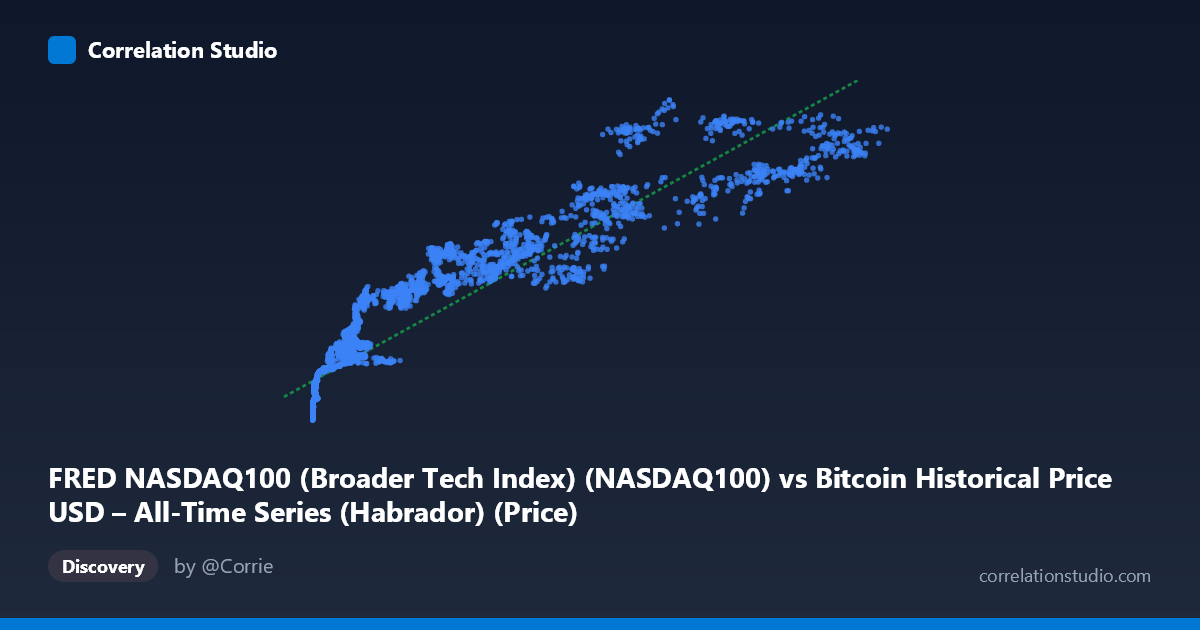
FRED NASDAQ100 (Broader Tech Index) (NASDAQ100) vs Bitcoin Historical Price USD – All-Time Series (Habrador) (Price)
- Pearson correlation (r)
- 0.9352
- Spearman correlation
- 0.9808
- p-value
- 0
- Sample size (n)
- 3970
- 95% confidence interval
- 0.9311 to 0.939
- Granger causality
- None
- Granger optimal lag
- 10
AI analysis
Analysis: Bitcoin Price vs. NASDAQ-100 Index
1. What the Visualization Reveals
The scatterplot shows a strong, positive, non-linear relationship between Bitcoin's historical price (X-axis) and the NASDAQ-100 index (Y-axis). The data pattern is distinctly curved rather than linear — at low Bitcoin prices (under ~$1,000), NASDAQ values cluster tightly between roughly 2,000–5,000, showing minimal sensitivity to Bitcoin's movements. As Bitcoin price increases into the tens of thousands, NASDAQ values rise more steadily, but with visibly increasing scatter/variance at the high end (e.g., Bitcoin ~$86,000–$95,000 corresponds to NASDAQ values ranging from ~20,400 to ~25,600). This suggests a relationship that resembles a logarithmic or power-law curve more than a straight line, since Bitcoin's range spans nearly 6 orders of magnitude (0.05 to 124,720) while NASDAQ's range spans less than one order of magnitude (1,767 to 27,306).
2. Strength, Direction, and Statistical Meaning
The correlation coefficient (r = 0.935) indicates a strong positive linear association, with r² = 0.875 meaning the linear model explains about 87.5% of the variance in NASDAQ-100 values based on Bitcoin price. The tight 95% confidence interval [0.931, 0.939] and p-value of 0 (effectively p < 0.0001) confirm this correlation is highly statistically significant and not due to sampling noise, especially given the large sample size (n=3,970). However, statistical significance and strength of correlation should not be conflated with causation. The Granger causality tests are critical here: neither direction shows significant predictive power (X→Y: p=0.85; Y→X: p=0.81) even at an optimal lag of 10 periods. This means that despite the strong contemporaneous correlation, past values of one series do not meaningfully help predict future values of the other — the relationship is likely driven by a shared underlying trend (e.g., both assets appreciating over the same long time period, 2010–2026) rather than one market mechanically leading the other.
3. Notable Patterns and Outliers
The data reveals at least two distinct regimes: a "low-Bitcoin" cluster (X < 1,000) where NASDAQ hovers narrowly around 2,200–5,800, and a "high-Bitcoin" regime (X 40,000) where NASDAQ climbs to 13,000–25,600. The transition between these regimes is not smooth — there's considerable vertical spread at high Bitcoin prices (e.g., $86,475 → NASDAQ 20,426 vs. $86,473 → NASDAQ 25,343), indicating that for similar Bitcoin prices, NASDAQ can vary substantially, likely reflecting different time periods with different macro conditions. This heteroscedasticity (variance increasing with X) violates a key assumption of simple linear regression and reinforces that a log-transform of Bitcoin price (or both variables) would likely produce a better-fitting, more homoscedastic model.
4. Confounding Factors and Caveats
The most significant confound is time itself. Both Bitcoin and the NASDAQ-100 have experienced substantial secular growth over the 2010–2026 window, driven by macro factors like near-zero interest rates (2010s), quantitative easing, growing tech-sector dominance, and increasing risk-asset speculation. This shared temporal trend can produce high correlation between virtually any two growing time series without genuine economic linkage — a classic spurious correlation risk in time-series analysis. The lack of Granger causality strongly supports this interpretation: it's not that Bitcoin drives NASDAQ or vice versa, but that both are responding to common macro liquidity/risk-appetite conditions. Additionally, the extreme skew in Bitcoin's distribution (mean 20,752 vs. median likely far lower, given the range starting at $0.05) means the correlation could be disproportionately influenced by the small number of very high-Bitcoin-price observations.
5. Actionable Insights and Further Investigation
Given the non-linear pattern, a log-log or semi-log regression (log(Bitcoin) vs. NASDAQ, or both logged) would likely yield a more accurate and interpretable model than the current linear fit. To disentangle genuine linkage from shared time trend, analysts should detrend both series (e.g., using returns/percentage changes instead of price levels) and re-test correlation and Granger causality on the detrended or differenced series — this is the standard approach to avoid spurious correlation in trending time series. Additionally, testing correlation within specific sub-periods (e.g., 2020–2022 bull market vs. 2022–2023 bear market) would reveal whether the relationship is stable or regime-dependent. Finally, incorporating a third variable — such as a broad liquidity indicator (M2 money supply) or risk-sentiment index (VIX) — as a control could help determine whether Bitcoin and NASDAQ are both proxies for a common "risk-on/risk-off" factor rather than being directly linked to one another.
X dataset: Bitcoin Historical Price USD – All-Time Series (Habrador)
Y dataset: FRED NASDAQ100 (Broader Tech Index)
Part of experiment: Bitcoin - Bitcoin Historical Price USD – All-Time Series (Habrador) vs FRED NASDAQ100 (Broader Tech Index)