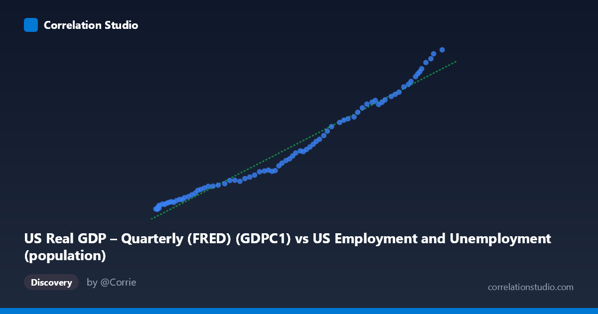
US Real GDP – Quarterly (FRED) (GDPC1) vs US Employment and Unemployment (population)
- Pearson correlation (r)
- 0.9857
- Spearman correlation
- 0.9994
- p-value
- 0
- Sample size (n)
- 79
- 95% confidence interval
- 0.9777 to 0.9909
- Granger causality
- None
- Granger optimal lag
- 10
AI analysis
Analysis: US Real GDP vs. US Employment Population
1. Overall Relationship
The scatterplot reveals a strong, positive, and nearly linear relationship between US Real GDP (quarterly, in billions of chained 2017 dollars) and the US employment/unemployment population measure. As GDP rises from approximately $103,000 to $273,000 (likely in billions), the employment population figure climbs correspondingly from roughly 2,183 to 23,548. The data points trace a remarkably tight upward arc across the full range, with very little scatter around the fitted regression line (y = 0.1168x − 10,858.4), indicating that these two variables have moved in close tandem across the 1947–2025 time coverage. The relationship is consistent across the entire observed range, with no dramatic breaks or reversals visible in the primary trend.
2. Correlation Strength and Statistical Significance
The correlation is exceptionally strong (r = 0.9859), and critically, the R² of 0.9719 means that 97.2% of the variance in the employment population measure is statistically explained by variation in Real GDP — leaving only 2.8% attributable to other factors within this bivariate framework. The 95% confidence interval for r [0.9779, 0.9910] is narrow and lies entirely at the high end of the scale, confirming this is not a fragile estimate — the true population correlation is almost certainly very high. The p-value of essentially zero (p ≈ 0) across n = 79 paired observations makes any chance explanation vanishingly unlikely. However, Granger causality tests tell a more nuanced story: neither direction (X→Y: F = 1.41, p = 0.206; Y→X: F = 1.56, p = 0.149) reaches statistical significance at conventional thresholds, even at the optimal lag of 10 periods (~2.5 years). This means that, while the two series are tightly correlated contemporaneously, neither reliably predicts the other's future values beyond what each series already predicts about itself — a crucial distinction between correlation and temporal causation.
3. Notable Patterns and Features
Examining the data points more closely, the relationship is not perfectly linear — there is a subtle convex curvature, particularly evident in the upper range where GDP values exceed ~230,000 and employment population values rise steeply (e.g., points near 268,571 / 23,082 and 273,653 / 23,548). This slight upward acceleration suggests the relationship may be better modeled with a polynomial or logarithmic functional form rather than a strict linear one. The lower end of the distribution (GDP ~103,000–130,000, employment population ~2,200–4,900) shows tightly clustered points corresponding to the post-WWII era, while the upper-right cluster represents the modern economy. There are no dramatic outliers that would distort the regression, though a few mid-range points (e.g., around GDP ~207,753 with employment 13,316) sit marginally above the fitted line, hinting at periods where employment grew faster than GDP growth would predict.
4. Confounding Factors and Interpretive Caveats
Several important caveats limit causal interpretation. Most critically, both series are strongly trended over time — they grow together largely because both reflect long-run economic expansion driven by population growth, technological progress, and capital accumulation. This introduces spurious correlation risk: two unrelated but upward-trending time series would also show high r values. The failure of Granger causality in both directions reinforces this concern — the apparent relationship may be substantially a shared trend artifact rather than a meaningful economic mechanism. Additionally, the unit mismatch deserves scrutiny: Real GDP is measured in billions of chained 2017 dollars while the Y-axis is labeled as "population" within the GDP dataset, suggesting this may reflect civilian labor force or total population figures cross-referenced from the employment dataset — the exact variable definition should be confirmed before drawing policy conclusions. Structural breaks (the 2008–09 financial crisis, 2020 COVID shock) are embedded in the data but may not be visually prominent due to the dominant long-run trend. The dataset also aggregates quarterly GDP with annual employment data (N=86, n=79), introducing temporal granularity mismatches that could affect dynamic analyses.
5. Actionable Insights and Further Investigation
Given the ambiguity around temporal causation, several follow-up analyses are warranted. First, detrend both series (e.g., using first differences or HP filtering) and retest the correlation — if r drops substantially, much of the observed relationship is trend-driven rather than cyclical comovement. Second, re-run Granger causality tests at shorter lag structures (1–4 quarters) to check whether the null result holds across all horizons, and consider vector autoregression (VAR) modeling to capture joint dynamics. Third, clarify the Y-axis variable definition precisely — if this is total civilian population, the relationship to GDP is mechanistically different than if it is employed persons or labor force participants. Fourth, introduce control variables (labor force participation rate, productivity indices, capital investment) to test whether GDP retains explanatory power in a multivariate framework. Finally, segment the analysis by economic regime (pre/post-1980 productivity slowdown, pre/post-2008) to determine whether the relationship has been structurally stable or whether the current high-r value masks important shifts in the GDP-employment nexus over the 78-year sample period.
X dataset: US Employment and Unemployment
Y dataset: US Real GDP – Quarterly (FRED)
Part of experiment: Yearly - US Employment and Unemployment vs US Real GDP – Quarterly (FRED)