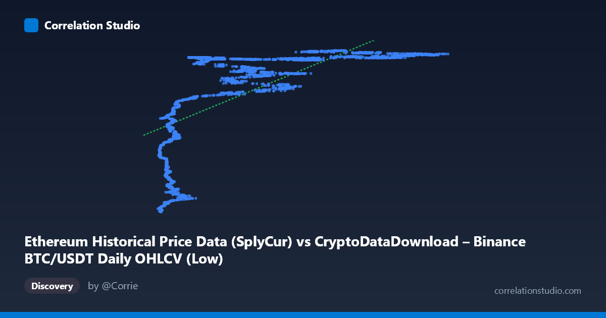
Ethereum Historical Price Data (SplyCur) vs CryptoDataDownload – Binance BTC/USDT Daily OHLCV (Low)
- Pearson correlation (r)
- 0.6741
- Spearman correlation
- 0.8254
- p-value
- 0
- Sample size (n)
- 3191
- 95% confidence interval
- 0.6547 to 0.6926
- Granger causality
- None
- Granger optimal lag
- 10
- Time coverage
- 2017-08-17 to 2026-05-20
AI analysis
Analysis: Ethereum Supply (SplyCur) vs. BTC/USDT Low Price
(Note: the axis labels appear mismatched with the described datasets — X is labeled "Ethereum Supply" but described as BTC/USDT data, while Y is labeled BTC/USDT Low but described as Ethereum metrics. The analysis below treats X and Y purely as the two numeric series provided, since the labels are internally inconsistent.)
1. What the Visualization Reveals
The scatterplot shows a positive but distinctly non-linear relationship between X and Y. Rather than a smooth linear trend, the data appears to cluster into a low-X/low-Y regime (X < ~15,000, Y clustered around 94–113 million) and a high-X/high-Y plateau (X ~20,000, Y saturating around 118–122 million). This pattern is characteristic of a logarithmic or saturating curve — Y rises steeply as X increases from its minimum, then flattens out and barely moves despite large further increases in X (e.g., X moving from 60,000 to 120,000 produces almost no change in Y).
2. Strength, Direction, and Statistical Confidence
The Pearson correlation (r = 0.674, r² = 0.454) indicates a moderate-to-strong positive linear association, but only 45% of the variance in Y is explained by a linear fit in X — meaning more than half of Y's variability is left unexplained by this simple model. The tight confidence interval [0.655, 0.693] and p ≈ 0 confirm this correlation is highly statistically significant and not due to sampling noise, given the large n (3,191). However, statistical significance here reflects the large sample size, not necessarily a strong or well-specified relationship — the CI tells us we're confident about the magnitude of r, not that r itself is high.
Critically, the Granger causality tests show no significant predictive direction in either direction (X→Y: p=0.91; Y→X: p=0.40). This strongly suggests the correlation is not driven by one variable temporally leading the other. Instead, both series likely share a common underlying driver (e.g., overall market growth, time trend, or a shared macro factor) rather than one causing the other in a lagged, dynamic sense.
3. Notable Patterns and Non-linearity
- Saturation/plateau effect: Y compresses into a narrow band (~118–122M) once X exceeds ~20,000, while below that threshold Y drops sharply and disperses widely (94M–113M). This is the hallmark of a logarithmic relationship, consistent with the note that Spearman ρ exceeds Pearson r — rank-order correlation captures the monotonic trend better than a straight line does. - Two distinct clusters: a "low regime" cluster (X≈3,700–20,000, Y≈94M–114M) with much more scatter, and a "high regime" cluster (X≈20,000–123,000, Y≈118M–122M) with very low scatter/variance. - No visible outliers breaking the overall monotonic pattern — the extremes (lowest X/lowest Y and highest X/highest Y) are consistent with the curve's endpoints, not anomalies. - The steep initial rise suggests diminishing returns: early increases in X are associated with large jumps in Y, but this effect rapidly weakens.
4. Confounding Factors and Caveats
- Shared time trend: Since both series span 2017–2026 and cryptocurrency markets have exhibited long-term secular growth/appreciation, both X and Y may simply be trending upward together over time (spurious correlation via a common time-based confound) rather than reflecting genuine bivariate dependence. - Autocorrelation: Daily financial/supply data is highly autocorrelated; the "n=3,191 independent pairs" assumption underlying the p-value is likely violated, meaning the true effective sample size is smaller and statistical significance is probably overstated. - Label ambiguity: The axis metadata is contradictory (mixing ETH supply with BTC price columns), which raises concern about data pipeline errors — this should be verified before drawing domain conclusions. - Non-linear model misspecification: Because the true relationship is saturating/logarithmic, the linear r² of 0.454 understates the true strength of association between the (transformed) variables.
5. Actionable Insights
- Re-fit with a logarithmic or power-law model (Y ~ a·ln(X) + b) — given the Spearman/Pearson discrepancy and visible saturation, this should substantially improve explained variance over the current linear R²=0.454. - Verify data labeling/joins — resolve the mismatch between stated column names and dataset descriptions before publishing conclusions. - Test cointegration rather than Granger causality on levels — since Granger causality on raw (likely non-stationary, trending) series is unreliable, consider differencing the data or testing for a shared stochastic trend (e.g., Engle-Granger or Johansen cointegration test). - Segment the analysis by regime — fit separate models to the low-X and high-X clusters, since the relationship's slope and variance behave very differently in each region. - Control for time explicitly — include a time/trend term or examine year-over-year correlation to determine whether the association survives after detrending, which would clarify whether this is a genuine bivariate relationship or a shared-growth artifact.
X dataset: CryptoDataDownload – Binance BTC/USDT Daily OHLCV
Y dataset: Ethereum Historical Price Data
Part of experiment: Bitcoin - CryptoDataDownload – Binance BTC/USDT Daily OHLCV vs Ethereum Historical Price Data