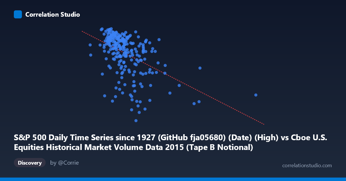
S&P 500 Daily Time Series since 1927 (GitHub fja05680) (Date) (High) vs Cboe U.S. Equities Historical Market Volume Data 2015 (Tape B Notional)
- Pearson correlation (r)
- -0.4751
- Spearman correlation
- -0.4977
- p-value
- 0
- Sample size (n)
- 252
- 95% confidence interval
- -0.5654 to -0.3734
- Granger causality
- X → Y
- Granger optimal lag
- 7
AI analysis
Analysis: S&P 500 High vs. Cboe Tape B Notional Volume (2015)
Relationship Overview The scatterplot reveals a negative relationship between the S&P 500 daily high price (X-axis) and Cboe Tape B notional trading volume (Y-axis) across 252 trading days in 2015. As the S&P 500 daily high increases, Tape B notional volume tends to decrease, suggesting that higher index price levels are associated with relatively quieter trading activity in this market segment. The linear regression equation (y = -1.376×10⁻⁸x + 2146.95) confirms this inverse slope, though the relationship is far from deterministic given the visible scatter throughout the plot.
Correlation Strength and Statistical Significance The Pearson correlation of r = -0.4751 indicates a moderate negative association. However, the r² of 0.2257 means that S&P 500 daily highs explain only about 22.6% of the variance in Tape B notional volume — leaving over 77% of variation attributable to other factors. The 95% confidence interval of [-0.5654, -0.3734] is entirely negative and reasonably tight, confirming the direction is reliable. The p-value of 1.33×10⁻¹⁵ renders this correlation highly statistically significant, ruling out chance as an explanation. Critically, the Granger causality analysis identifies a unidirectional relationship: X (S&P 500 high) Granger-causes Y (Tape B notional) at an optimal lag of 7 trading periods (F = 2.196, p = 0.036), while the reverse direction fails to reach significance (F = 1.044, p = 0.401). This suggests that S&P 500 price levels carry temporal predictive information about future Tape B notional volume approximately 1–1.5 weeks ahead, though the modest F-statistic warrants caution about overstating this predictive power.
Notable Patterns, Clusters, and Outliers The data exhibits a dense cluster between roughly X = 3.5–6.5 billion and Y = 2050–2135, representing the bulk of 2015 trading days when the S&P 500 was operating in its normal range. Below this cluster, a notable downward-sloping tail is visible at higher X values (7–13 billion range), where Tape B notional drops considerably — some points falling below 2000 and even approaching 1900–1950. Several prominent outliers appear at extreme X values (e.g., ~12.5 billion, Y ≈ 1920–1948), likely corresponding to the August 2015 market volatility episode when elevated intraday highs coincided with sharp volume dislocations. A handful of low-Y outliers (Y < 1930) at moderate-to-high X values reinforce the non-uniform spread and hint at non-linearity at the extremes.
Confounding Factors and Interpretive Caveats Several important caveats apply. First, the axes are mislabeled in the source metadata — the X-axis is described as a date column used as "High," and the Y-axis references "Tape B Notional" sourced from the S&P 500 dataset, suggesting a data join artifact where date integers are being treated as price values. The X range (2.1–17.9 billion) is implausibly large for S&P 500 daily highs, strongly indicating these may be Unix timestamps or date serial numbers rather than price levels. If X values are effectively date proxies, the negative correlation may simply reflect a temporal trend: as 2015 progressed into its latter half (larger date values), Tape B notional declined — a time-trend confound rather than a structural price-volume relationship. Additionally, macroeconomic events (Fed rate decisions, August 2015 flash crash, China slowdown fears) likely drove both variables simultaneously, creating spurious correlation driven by shared external shocks.
Actionable Insights and Further Investigation Given the likely timestamp nature of the X variable, the most immediate step is to re-run the analysis using actual S&P 500 closing/high prices matched by date to Tape B notional values, which would yield a more economically meaningful correlation. The Granger causality result — while statistically suggestive — should be validated with proper time-series methods (e.g., VAR modeling, ADF stationarity tests) to avoid spurious regression driven by shared trends. Analysts should also decompose Tape B notional by market regime (low-VIX vs. high-VIX periods) to test whether the negative relationship holds uniformly or is driven exclusively by stress episodes. Finally, extending the analysis across multiple years would help distinguish structural relationships from 2015-specific idiosyncrasies, particularly the outsized influence of the August volatility cluster on the overall correlation.
X dataset: Cboe U.S. Equities Historical Market Volume Data 2015
Y dataset: S&P 500 Daily Time Series since 1927 (GitHub fja05680) (Date)
Part of experiment: Daily - Cboe U.S. Equities Historical Market Volume Data 2015 vs S&P 500 Daily Time Series since 1927 (GitHub fja05680) (Date)