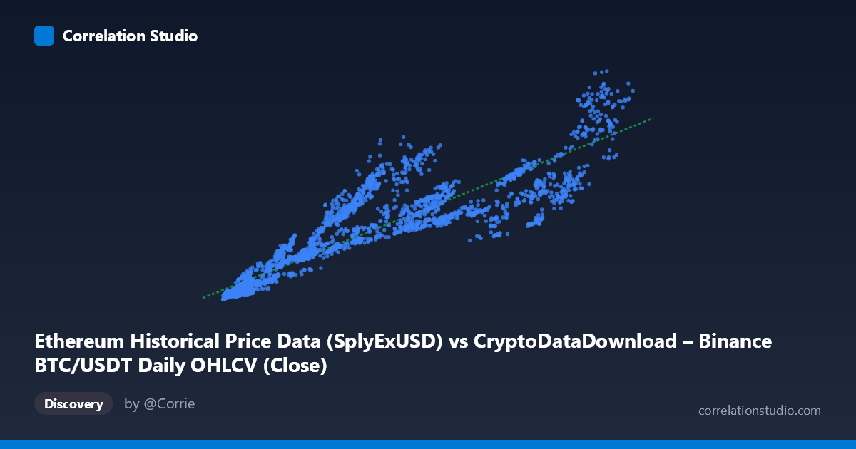
Ethereum Historical Price Data (SplyExUSD) vs CryptoDataDownload – Binance BTC/USDT Daily OHLCV (Close)

Pearson correlation (r): 0.9056
Spearman correlation: 0.944
p-value: 0
Sample size (n): 3191
95% confidence interval: 0.8991 to 0.9116
Granger causality: None
Granger optimal lag: 10

AI analysis

Analysis: Ethereum Supply/Price Metric vs. Bitcoin Price

1. Overview of the Relationship

The scatterplot displays a strong positive association between the X variable (labeled as an Ethereum-related metric, though the column name references "SplyExUSD" — Supply on Exchanges) and Y (BTC/USDT closing price). As X increases from roughly 3,200 to 124,600, Y rises correspondingly from ~$1.4B to ~$95.6B. The data points trace a generally upward-sloping band, consistent with the fitted linear model: y = 556,502x + 3.53B. However, close inspection reveals the relationship is not perfectly linear — there's noticeable fanning and scatter, especially at higher X values, suggesting the true relationship may involve non-linear components or additional volatility at scale.

2. Strength, Direction, and Statistical Confidence

The correlation coefficient (r = 0.906) indicates a strong positive linear relationship, with r² = 0.820 meaning approximately 82% of the variance in Y is statistically explained by X — a substantial figure, though it leaves ~18% attributable to other factors or noise. The 95% confidence interval [0.899, 0.912] is tight, reflecting the large sample size (n=3,191) and giving high confidence that the true population correlation is robust and non-zero (p ≈ 0).

Critically, Granger causality tests show no significant predictive direction in either direction (X→Y: p=0.877; Y→X: p=0.825). This is an important caveat: despite the strong contemporaneous correlation, neither variable reliably predicts future values of the other over time. This suggests the relationship is likely driven by a shared underlying factor (e.g., overall crypto market sentiment, macro liquidity conditions, or a common time trend) rather than one asset mechanically leading the other.

3. Notable Patterns and Outliers

Several features stand out: - Heteroscedasticity: Variance in Y appears to increase with X — at low X (~4,000–10,000), Y values cluster tightly between $2–13B, but at high X (~80,000–110,000), Y ranges widely from $27B to $81B. - Possible clustering/regime shifts: Points like (36,445 → $34.4B) and (39,020 → $39.4B) sit notably above the trend line compared to neighboring X values, hinting at distinct market regimes or bull-run periods where price decoupled from the X metric. - Compression at low end: Below X=15,000, points are densely packed with a steeper apparent slope, suggesting possible non-linear (e.g., logarithmic) dynamics that a simple linear fit doesn't fully capture.

4. Confounding Factors and Caveats

Both variables are derived from crypto market data spanning 2017–2026, a period marked by extreme volatility, multiple bull/bear cycles, and structural market changes (regulatory shifts, exchange dynamics, ETF approvals, etc.). Key concerns: - Spurious correlation risk: Two trending time series (both generally rising over years) will show high correlation even without causal linkage — this is a classic time-series pitfall, reinforced by the null Granger causality result. - Non-stationarity: Neither series likely has constant mean/variance over time, violating assumptions needed for correlation to imply meaningful structural relationship. - Dataset mismatch: The metadata is inconsistent (X labeled as Ethereum supply metric, Y labeled as BTC price, but described elsewhere as Ethereum price/network data) — this warrants verification before drawing asset-specific conclusions.

5. Recommendations for Further Investigation

1. Verify variable identity — resolve the labeling ambiguity between BTC and ETH data before making asset-specific claims. 2. Test for cointegration (e.g., Engle-Granger or Johansen test) rather than relying on simple correlation, given the non-stationary, trending nature of crypto prices. 3. Detrend or difference the series (e.g., use log returns instead of levels) to check if the correlation persists after removing shared trend — this will reveal whether the relationship is genuine or an artifact of co-movement with the broader market. 4. Segment by market regime (bull/bear/sideways) to see if the r² and slope are stable or regime-dependent, given the apparent outlier clustering. 5. Introduce a third variable (e.g., total crypto market cap, DXY, or interest rates) to test whether both X and Y are jointly driven by a common macro factor, which would explain the strong correlation without causality.

X dataset: CryptoDataDownload – Binance BTC/USDT Daily OHLCV

Y dataset: Ethereum Historical Price Data

Part of experiment: Bitcoin - CryptoDataDownload – Binance BTC/USDT Daily OHLCV vs Ethereum Historical Price Data