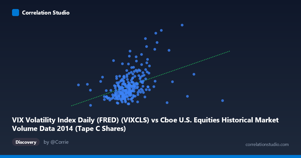
VIX Volatility Index Daily (FRED) (VIXCLS) vs Cboe U.S. Equities Historical Market Volume Data 2014 (Tape C Shares)
- Pearson correlation (r)
- 0.401
- Spearman correlation
- 0.4186
- p-value
- 0
- Sample size (n)
- 252
- 95% confidence interval
- 0.2919 to 0.4998
- Granger causality
- None
- Granger optimal lag
- 1
AI analysis
Analysis: VIX Volatility Index vs. Cboe Tape C Share Volume (2014)
Relationship Overview The scatterplot reveals a moderate positive relationship between Cboe U.S. equities market volume (Tape C shares, X-axis) and the VIX Volatility Index (Y-axis) across 252 trading days in 2014. The linear regression equation (y = 4.27×10⁻⁸x + 8.47) confirms that as daily share volume increases, VIX tends to rise — a directionally intuitive finding, since elevated market anxiety typically drives both higher volatility readings and increased trading activity. However, the relationship is far from clean, with considerable scatter throughout the distribution, and the bulk of observations clustering in the 100–160 million share range with VIX values between roughly 11 and 17.
Correlation Strength and Statistical Significance The correlation of r = 0.40 indicates a moderate positive association, but the explanatory power is limited: r² = 0.161 means only 16.1% of the variance in VIX is explained by Tape C volume, leaving roughly 84% attributable to other factors. The 95% confidence interval of [0.29, 0.50] is meaningfully above zero and relatively tight given the sample size of 252, and the p-value of 3.74×10⁻¹¹ confirms this correlation is highly unlikely to be a chance artifact. Critically, however, Granger causality tests find no significant predictive direction in either direction (X→Y: F=0.89, p=0.35; Y→X: F=0.55, p=0.46), meaning that past volume does not reliably forecast future VIX and vice versa at a one-period lag. This distinguishes statistical association from temporal predictability — the variables move together but neither leads the other in a consistently exploitable way.
Notable Patterns, Clusters, and Outliers Several features stand out beyond the central cluster. A small but prominent group of high-VIX outliers (VIX ≥ 20–26) appears at moderate-to-high volume levels (roughly 150–200 million shares), likely corresponding to specific volatility spikes in 2014 — most plausibly the October 2014 equity correction or geopolitical stress events. Conversely, there are low-VIX observations (≈10.5–12) scattered across a wide volume range, suggesting that calm periods can occur at both light and heavy trading volumes. One notable low-volume outlier (~52 million shares, VIX ~14.4) sits far left of the main cluster, possibly reflecting a holiday-shortened session or data anomaly. The scatter's fan-like spread widening at higher volume values hints at mild heteroscedasticity — VIX becomes more variable as volume grows, which can slightly inflate the linear correlation estimate.
Confounding Factors and Caveats Several important caveats apply. First, reverse causality is plausible: VIX spikes may cause volume surges (fear-driven selling/hedging) just as much as volume predicts VIX, which the Granger results reflect. Second, Tape C represents only a subset of total U.S. equity volume (NYSE Arca-listed securities), so this isn't a complete market picture. Third, 2014 was a relatively low-volatility year overall (VIX averaged ~14), meaning the sample is not representative of crisis regimes — the relationship may behave very differently in high-stress periods like 2008 or 2020. Fourth, day-of-week and seasonal effects (e.g., lower volume on Fridays or around holidays) could create spurious co-movement patterns. Finally, the axes in the dataset metadata appear to have been swapped in labeling (VIX values align with Y-axis ranges 10–26, while share counts align with X-axis values in the hundreds of millions), which warrants verification before drawing firm conclusions.
Actionable Insights and Further Investigation Practitioners should avoid using daily Tape C volume alone as a VIX forecasting signal given the weak Granger results and low r². More productive next steps would include: (1) testing multi-day lagged relationships (lags 1) or intraday volume patterns, which may reveal predictive structure obscured at the daily level; (2) segmenting the analysis by market regime (low vs. high VIX environments) to test whether the correlation strengthens nonlinearly during stress periods; (3) incorporating total consolidated volume across all tapes rather than Tape C alone; and (4) applying a log transformation to both variables to address heteroscedasticity and potentially improve model fit. For risk management applications, this relationship could still serve as a weak confirmatory signal within a broader multi-factor volatility model, even if it lacks standalone predictive power.
X dataset: Cboe U.S. Equities Historical Market Volume Data 2014
Y dataset: VIX Volatility Index Daily (FRED)
Part of experiment: Daily - Cboe U.S. Equities Historical Market Volume Data 2014 vs VIX Volatility Index Daily (FRED)