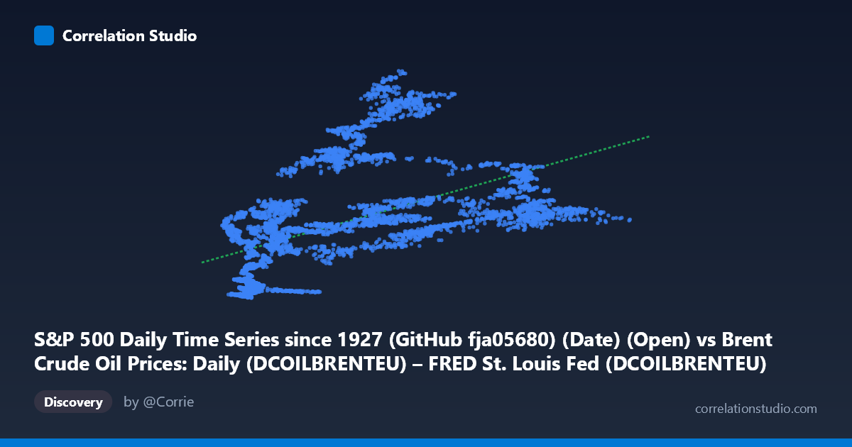
S&P 500 Daily Time Series since 1927 (GitHub fja05680) (Date) (Open) vs Brent Crude Oil Prices: Daily (DCOILBRENTEU) – FRED St. Louis Fed (DCOILBRENTEU)
- Pearson correlation (r)
- 0.5236
- Spearman correlation
- 0.6822
- p-value
- 0
- Sample size (n)
- 7266
- 95% confidence interval
- 0.5067 to 0.54
- Granger causality
- None
- Granger optimal lag
- 1
- Time coverage
- 1987-05-20 to 2019-12-23
- Recomputed on refreshed data
- 2026-10-22 (r was 0.5236)
AI analysis
Analysis: Brent Crude Oil Price vs. S&P 500 Index (1987–2019)
1. Overall Relationship The scatterplot reveals a positive but notably dispersed relationship between Brent crude oil prices (X-axis, USD/barrel) and the S&P 500 index level (Y-axis). As oil prices rise from roughly $10 to $144/barrel, S&P 500 values trend upward from ~$225 to ~$3,226. However, the wide vertical spread at virtually every X value makes it immediately clear that this is far from a deterministic relationship — at oil prices around $60–70/barrel, for instance, S&P 500 values range dramatically from below $1,000 to above $3,200, reflecting the fact that both variables were largely moving together through time as part of broader economic expansion rather than one directly driving the other.
2. Correlation Strength and Statistical Framing The Pearson correlation of r = 0.538 indicates a moderate positive association, but the explanatory power is modest: R² = 0.289 means only 28.9% of S&P 500 variance is explained by Brent crude prices, leaving over 71% attributable to other forces. The 95% confidence interval of [0.522, 0.554] is tight given the large sample (n = 8,140), confirming the estimate is precise and stable — but precision does not imply importance. The p-value of effectively zero confirms this is not a chance finding at this sample size. Critically, Granger causality tests find no significant predictive directionality in either direction (X→Y: F = 0.90, p = 0.34; Y→X: F = 0.86, p = 0.35), meaning that knowing today's oil price does not meaningfully improve forecasts of tomorrow's S&P 500, and vice versa. This strongly undermines any causal narrative and reframes the correlation as largely coincidental co-movement through shared macroeconomic time trends.
3. Notable Patterns, Clusters, and Non-Linearity Several structural features stand out in the data. A dense cluster of low-X, low-to-moderate-Y points appears in the $10–$30 oil range, corresponding to the late 1980s through mid-1990s when both oil and equity prices were relatively low. A second, more dispersed cluster emerges in the $50–$90 oil range with highly variable S&P values, reflecting the 2000s and 2010s when oil spiked while equities experienced both the dot-com crash and the post-2009 bull run — producing enormous vertical scatter. The hint that Spearman ρ exceeds Pearson r is important: it suggests the monotonic rank relationship is stronger than the linear one, pointing toward a logarithmic or polynomial fit being more appropriate. At extreme oil prices (above $100/barrel), S&P values do not continue rising proportionally, consistent with diminishing or even negative marginal effects of very high oil prices on equities. Several outliers exist at high X values (~$130–$144) paired with moderate Y values (~$1,200–$1,400), likely representing the 2008 oil price spike coinciding with the financial crisis equity collapse.
4. Confounding Factors and Caveats The most significant caveat is that both series are non-stationary time series — they both trend upward over the 1987–2019 period due to inflation, economic growth, and dollar debasement. This shared time trend is likely responsible for much of the observed correlation, a classic spurious correlation problem. The Granger causality results, which work on the differenced/level relationship with a lag structure, appropriately find no meaningful temporal link, reinforcing this interpretation. Additional confounders include: global GDP growth driving both energy demand and corporate earnings simultaneously; monetary policy cycles affecting both asset classes; and major structural breaks (1990 Gulf War, 1997 Asian crisis, 2001 dot-com bust, 2008 financial crisis, 2014–2016 oil glut) that create regime-dependent relationships. The linear regression equation (y = 11.52x + 650.70) should be treated skeptically given the non-linearity signal and the spurious trend concern.
5. Actionable Insights and Further Investigation Practitioners should not use crude oil prices as a standalone predictor of S&P 500 levels, given the absent Granger causality and low R². More productive next steps would include: (a) testing the relationship on first differences or percentage returns rather than price levels to remove the shared time trend and test genuine co-movement; (b) fitting a logarithmic or polynomial regression as suggested by the Spearman-Pearson divergence; (c) segmenting the analysis by economic regime (expansion vs. recession, pre/post-2008) since the oil-equity relationship is known to flip sign depending on whether oil shocks are supply- or demand-driven; and (d) incorporating control variables such as real GDP growth, the VIX, or dollar index to partial out shared macro drivers. A rolling-window correlation analysis would also reveal whether the relationship has strengthened, weakened, or reversed across decades — likely exposing that the aggregate correlation masks substantial structural instability.
X dataset: Brent Crude Oil Prices: Daily (DCOILBRENTEU) – FRED St. Louis Fed
Y dataset: S&P 500 Daily Time Series since 1927 (GitHub fja05680) (Date)
Part of experiment: Daily - Brent Crude Oil Prices: Daily (DCOILBRENTEU) – FRED St. Louis Fed vs S&P 500 Daily Time Series since 1927 (GitHub fja05680) (Date)