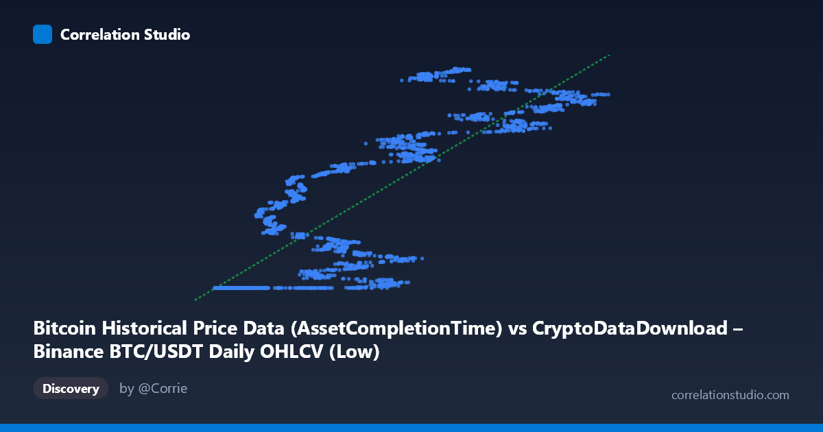
Bitcoin Historical Price Data (AssetCompletionTime) vs CryptoDataDownload – Binance BTC/USDT Daily OHLCV (Low)
- Pearson correlation (r)
- 0.8546
- Spearman correlation
- 0.89
- p-value
- 0
- Sample size (n)
- 3191
- 95% confidence interval
- 0.845 to 0.8637
- Granger causality
- None
- Granger optimal lag
- 10
AI analysis
Analysis of Bitcoin Price Data Correlation
1. What the Visualization Reveals
This scatterplot is somewhat unusual in that both axes derive from essentially the same underlying phenomenon: Bitcoin price. The X-axis appears to represent a timestamp/completion metric tied to BTC price data, while the Y-axis is the daily "Low" price from Binance OHLCV data. The plot reveals a clustered, non-linear pattern rather than a clean linear scatter — with a dense cluster of points around Y≈1,614,337,000 across a wide range of low X values (roughly 3,700–35,000), followed by a steep, more dispersed climb in Y as X increases beyond ~40,000.
2. Strength, Direction, and Uncertainty
The correlation coefficient (r = 0.855) indicates a strong positive relationship, with r² = 0.730 meaning about 73% of the variance in Y is statistically explained by X — a substantial but not complete linkage, leaving roughly 27% of variance driven by other factors or non-linear dynamics. The tight confidence interval [0.845, 0.864] combined with p ≈ 0 confirms this relationship is highly statistically robust and not a product of sampling noise, given the large N (3,191). However, statistical significance here reflects the strength of association, not causation. Critically, the Granger causality tests show no significant predictive direction in either direction (X→Y: p=0.35; Y→X: p=0.19) at the optimal 10-period lag. This means neither series reliably "leads" the other in time — despite the strong correlation, you cannot use one to forecast the other's future movements. This is a classic case of contemporaneous correlation without temporal causality.
3. Notable Patterns and Outliers
The most striking feature is the "floor" cluster: many points sit at nearly constant Y (~1,614,337,000–1,614,338,000) despite X ranging broadly from ~3,700 to ~35,000. This suggests a data artifact — possibly a placeholder, minimum timestamp, or early-period value that repeats before the data series "activates" and begins tracking price movement more dynamically. Beyond this cluster, the relationship becomes much steeper and more variable, with Y values jumping to 1.6–1.78 billion as X increases past ~40,000–60,000, indicating a regime change or non-linear (possibly logarithmic or threshold) relationship rather than a uniform linear trend across the full range.
4. Confounding Factors and Caveats
Given both variables originate from the same Bitcoin price dataset (one as a timestamp-like field, the other as a price low), this correlation may be structurally mechanical rather than economically meaningful — e.g., if X encodes time progression and Bitcoin price has trended upward over 2017–2026, the correlation could simply reflect a shared time trend (spurious correlation via a common driver: calendar time/market maturation). The clustering at a fixed Y value for many X points also suggests data quality issues, possible duplicate records, or an artifact of how "AssetCompletionTime" was encoded, which could bias the regression fit.
5. Actionable Recommendations
1. Clarify the X variable's actual meaning — confirm whether "AssetCompletionTime" is a true timestamp or a derived numeric field, as this determines whether the relationship is meaningful or tautological. 2. Investigate the flat cluster — isolate and examine the ~1,614,337,000 Y-value cluster to determine if it represents a data loading artifact, an early/inactive period, or legitimate low-volatility price action. 3. Test non-linear models (log-log, piecewise/segmented regression) given the apparent regime shift around X≈35,000–40,000, which likely fits better than the current linear model (slope 1459.11). 4. De-trend for time before drawing causal conclusions — control for calendar time or use returns/differences rather than levels, since both series may simply reflect Bitcoin's long-term bull trend. 5. Treat the Granger result as decisive: despite the strong r², do not use this relationship for predictive/trading purposes — the lack of significant lead-lag structure means it's likely a correlation of common trend rather than a forecastable dynamic.
X dataset: CryptoDataDownload – Binance BTC/USDT Daily OHLCV
Y dataset: Bitcoin Historical Price Data
Part of experiment: Bitcoin - CryptoDataDownload – Binance BTC/USDT Daily OHLCV vs Bitcoin Historical Price Data