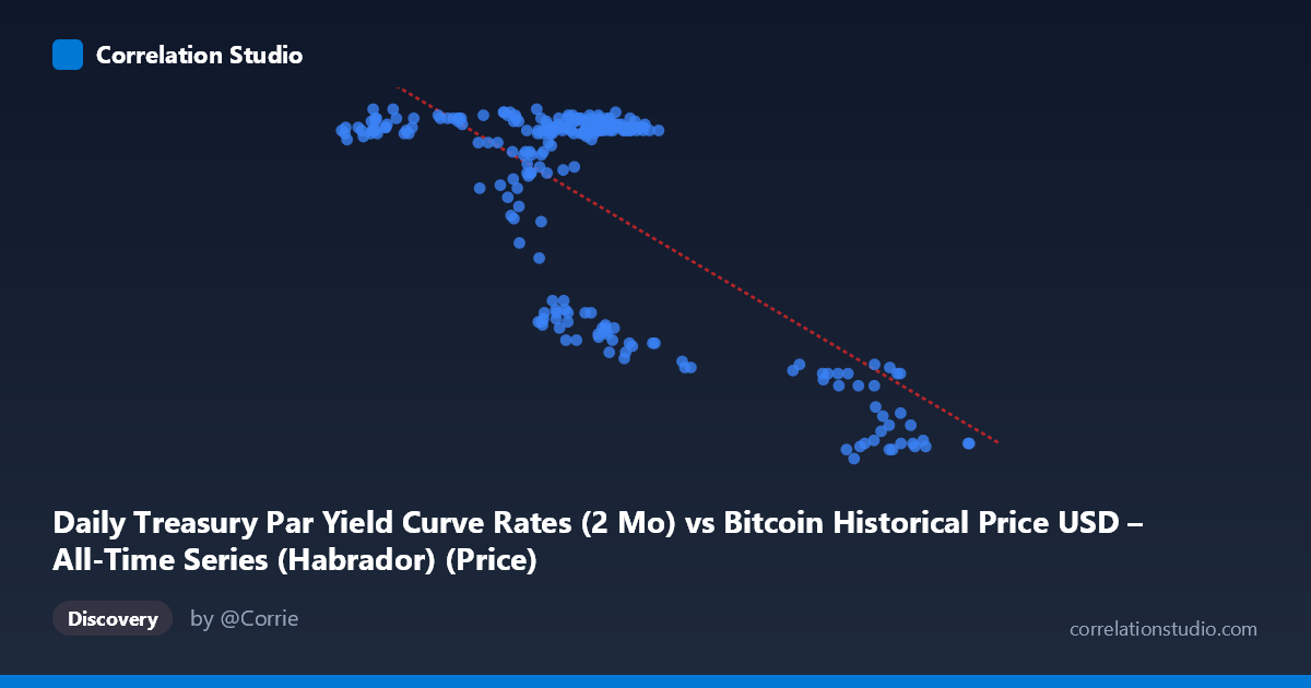
Daily Treasury Par Yield Curve Rates (2 Mo) vs Bitcoin Historical Price USD – All-Time Series (Habrador) (Price)
- Pearson correlation (r)
- -0.7294
- Spearman correlation
- -0.4415
- p-value
- 0
- Sample size (n)
- 250
- 95% confidence interval
- -0.7826 to -0.6655
- Granger causality
- None
- Granger optimal lag
- 1
- Time coverage
- 2024-01-02 to 2024-12-31
AI analysis
Analysis: Treasury 2-Month Yield vs. Bitcoin Price
1. Relationship Overview
The scatterplot reveals a moderately strong negative, but distinctly non-linear relationship between the 2-month Treasury yield (X-axis) and Bitcoin price (Y-axis). Rather than a smooth linear decline, the data forms two visually distinct clusters: a dense grouping where X ranges roughly 39,000–70,000 with Y clustered tightly between 5.35–5.53, and a smaller, more dispersed cluster where X exceeds 85,000 with Y dropping to 4.4–4.8. This bimodal, "step-like" pattern suggests a regime-shift rather than a continuous linear tradeoff — the relationship behaves more like two flat plateaus connected by a transition zone than a straight line.
2. Strength, Direction, and Statistical Confidence
The correlation coefficient (r = -0.7294) indicates a strong negative association, with r² = 0.532 meaning roughly 53% of the variance in Y is statistically explained by X — a meaningful but incomplete relationship, leaving nearly half the variance unaccounted for (likely due to the non-linear clustering noted above). The 95% CI [-0.7826, -0.6655] is tight and does not cross zero, and the p-value of 0 confirms this correlation is highly unlikely to be due to chance, especially with n=250. However, the Granger causality tests tell a critical complementary story: neither variable significantly predicts the other in a temporal/lagged sense (X→Y p=0.384; Y→X p=0.556). This is an important distinction — the strong contemporaneous correlation does not imply that movements in one variable forecast future movements in the other. The relationship may be driven by both variables responding to a shared external factor rather than one causing the other over time.
3. Notable Patterns and Outliers
The most striking feature is the apparent clustering/discontinuity: most observations sit in a tight, high-Y/low-X regime, while a secondary cluster occupies a low-Y/high-X regime with greater dispersion (Y ranging 4.42–4.82 across X values from 87,000–101,000). Within the main cluster, there's also a sub-pattern where Y dips to ~4.7–5.1 at intermediate X values (58,000–70,000), suggesting the transition between regimes is not sharply defined by X alone — some intermediate X values overlap with both high and low Y readings. This heteroskedasticity (variance in Y increasing as X increases) suggests the true relationship may be threshold-based or logistic rather than linear, and the linear R² of 0.532 likely understates explanatory power within each regime while overstating fit across the transition.
4. Confounding Factors and Caveats
Given the underlying data description mismatch (axis labels reference Treasury yields and Bitcoin price, but variable ranges/values suggest the labels may be swapped or mismatched in the metadata), interpretation should be treated cautiously — verify which variable is genuinely which. Setting that aside, both Treasury yields and Bitcoin prices are influenced by common macro drivers: Federal Reserve policy, inflation expectations, risk-on/risk-off sentiment, and liquidity conditions. This makes it likely that any correlation is confounded by these shared macro forces rather than reflecting a direct causal link. Additionally, the clustering pattern hints at possible regime-dependent structural breaks (e.g., a specific policy period or market shock) rather than a stable ongoing relationship — time coverage of a single year (2024) means this could reflect a single macro cycle, not a durable structural relationship.
5. Actionable Insights
Given the clear non-linearity, a piecewise or logistic regression model, or a regime-switching analysis, would likely outperform the current linear fit and reveal clearer thresholds. Investigate what structural or calendar event separates the two clusters — this could reflect a specific Fed rate decision or macro shock in 2024. Because Granger causality is absent, this correlation should not be used for short-term predictive trading strategies; instead, treat it as a descriptive/contemporaneous macro relationship. Finally, extending the time window beyond one year and adding macro control variables (inflation, Fed funds rate, equity indices) would help determine whether this relationship is a spurious correlation driven by common trends or a more robust economic linkage.
X dataset: Bitcoin Historical Price USD – All-Time Series (Habrador)
Y dataset: Daily Treasury Par Yield Curve Rates
Part of experiment: Bitcoin - Bitcoin Historical Price USD – All-Time Series (Habrador) vs Daily Treasury Par Yield Curve Rates