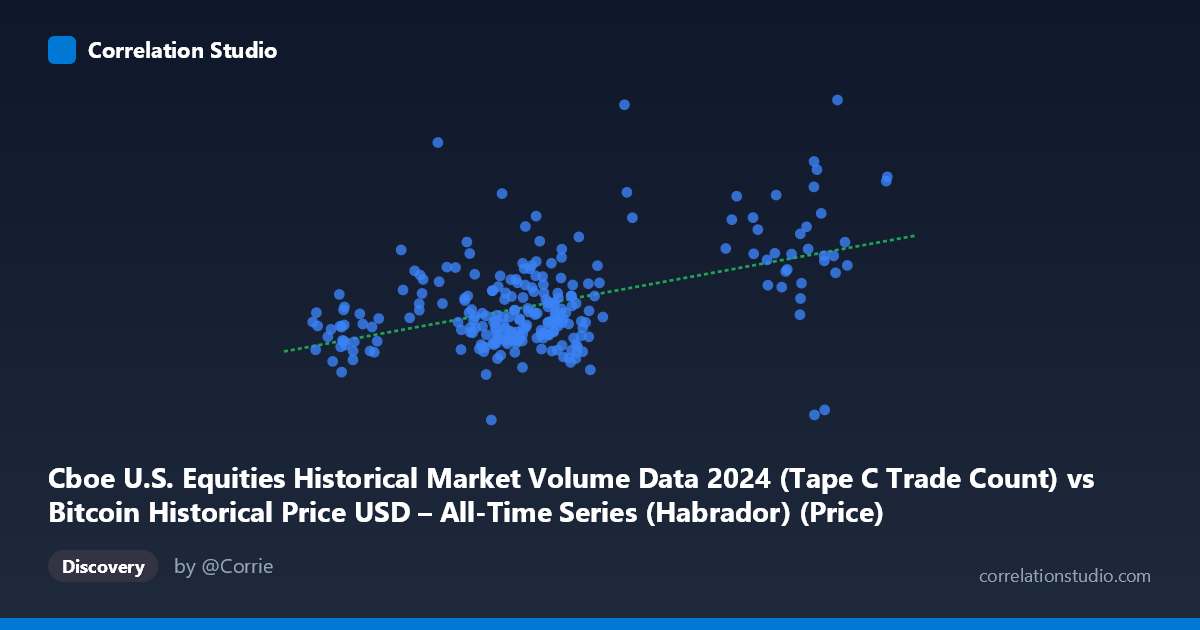
Cboe U.S. Equities Historical Market Volume Data 2024 (Tape C Trade Count) vs Bitcoin Historical Price USD – All-Time Series (Habrador) (Price)
- Pearson correlation (r)
- 0.4829
- Spearman correlation
- 0.3486
- p-value
- 0
- Sample size (n)
- 252
- 95% confidence interval
- 0.3821 to 0.5723
- Granger causality
- None
- Granger optimal lag
- 10
AI analysis
Analysis: Trade Count vs. Bitcoin Price Relationship
1. What the Visualization Reveals
The scatterplot shows a moderate positive relationship between Cboe Tape C trade counts and Bitcoin's daily USD price throughout 2024. Most observations cluster tightly in the X range of 55,000–72,000 trades with corresponding Bitcoin prices between roughly $1.6M–$2.4M (note: these Y values appear unusually large for BTC/USD, suggesting a possible unit or scaling issue in the dataset—see caveats below). A smaller subset of points extends to higher trade counts (96,000–102,000), and these do not show a proportionally stronger price relationship, indicating the association weakens or becomes noisy at the extremes.
2. Strength, Direction, and Predictive Value
The correlation coefficient (r = 0.483) indicates a moderate positive linear relationship, but the r² of 0.233 reveals that only about 23% of the variance in Bitcoin price is explained by trade count—leaving over three-quarters of price movement attributable to other factors. The 95% confidence interval [0.382, 0.572] is reasonably tight given n=252, and the extremely small p-value (4.4×10⁻¹⁶) confirms this correlation is highly statistically significant and not due to chance. However, statistical significance here reflects sample size and consistency, not practical strength—a moderate r² should temper any expectation that trade count is a reliable standalone predictor of price.
Critically, the Granger causality tests show no significant predictive direction in either direction (X→Y: p=0.232; Y→X: p=0.498). This means that despite the contemporaneous correlation, neither variable helps forecast future values of the other when using past values with a 10-period lag. This is an important distinction: the two series move together to some degree, but trade count doesn't temporally lead price changes, nor vice versa. This suggests the relationship may be driven by a shared external factor rather than a lead-lag causal mechanism.
3. Notable Patterns and Outliers
Several points stand out: - (53991.46, 2801223.32) is a clear high-Y outlier relative to its X value, sitting well above the regression line. - (60173.92, 1260223.79) is a low-Y outlier — lowest price in the sample despite a mid-range X. - The cluster of high-X points (96,000–101,100) shows inconsistent Y values (ranging from ~1.3M to ~2.4M), suggesting trade count alone doesn't reliably predict price direction at high volumes—this weakens the linear fit in the upper X range and hints at possible non-linearity or regime-dependent behavior. - The bulk of the data (X: 55,000–72,000) shows a loosely scattered cloud rather than a tight linear band, consistent with the modest r².
4. Confounding Factors and Caveats
Several concerns warrant caution: - Unit/scale mismatch: Bitcoin's actual 2024 price range was roughly $40,000–$108,000, not $1.26M–$3.04M as shown. This suggests either a data transformation, currency multiplier, or column mislabeling occurred—possibly the Y-axis reflects a different scaled metric or the X/Y columns were swapped from their dataset descriptions. This should be resolved before drawing economic conclusions. - Spurious correlation risk: Both Bitcoin price and equity trade volume can trend upward over a calendar year due to broader macro conditions (risk-on sentiment, liquidity cycles, rate expectations), creating correlated trends without direct causal linkage—consistent with the null Granger result. - Non-synchronized markets: Cboe equity trade counts and Bitcoin prices operate in different market structures (traditional equities vs. crypto), and any relationship is more likely mediated by common macro drivers (Fed policy, risk appetite) than direct interaction.
5. Suggested Next Steps
1. Verify data integrity: Confirm the axis labels and units match the actual source columns—current Y-values don't align with known BTC price history. 2. Test for shared confounders: Introduce macro variables (VIX, Fed rate decisions, overall equity index volume) as controls to see if the X-Y correlation diminishes, confirming a common-driver hypothesis. 3. Segment analysis: Separately examine the high-trade-count cluster (95,000) to understand why price variance increases there—possibly indicative of high-volatility market days. 4. Explore non-linear/lagged models: Given the null Granger result at lag 10, test shorter lags (1–5 days) or non-linear (e.g., polynomial, mutual information) relationships, since real-world market correlations often operate on shorter timescales.
X dataset: Bitcoin Historical Price USD – All-Time Series (Habrador)
Y dataset: Cboe U.S. Equities Historical Market Volume Data 2024
Part of experiment: Bitcoin - Bitcoin Historical Price USD – All-Time Series (Habrador) vs Cboe U.S. Equities Historical Market Volume Data 2024