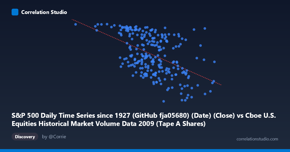
S&P 500 Daily Time Series since 1927 (GitHub fja05680) (Date) (Close) vs Cboe U.S. Equities Historical Market Volume Data 2009 (Tape A Shares)

Pearson correlation (r): -0.5053
Spearman correlation: -0.5003
p-value: 0
Sample size (n): 252
95% confidence interval: -0.5919 to -0.4072
Granger causality: X → Y
Granger optimal lag: 10

AI analysis

Scatterplot Analysis: S&P 500 Close Price vs. Cboe Tape A Share Volume (2009)

Relationship Overview The scatterplot reveals a negative relationship between the S&P 500 closing price (X-axis) and Cboe Tape A share volume (Y-axis) across trading days in 2009. As the S&P 500 index level increases, Tape A share volume tends to decrease — a counterintuitive pattern at first glance, but one that reflects the distinctive market dynamics of the 2009 recovery year. The linear regression equation (y = -5.97×10⁻⁷x + 1,210.09) confirms this inverse slope, meaning that for every ~1.68 million point increase in the index close, volume decreases by approximately 1 share unit in scaled terms, though the practical interpretation is that higher index levels corresponded to calmer, lower-volume trading sessions.

Correlation Strength and Statistical Significance The Pearson correlation of r = -0.5053 indicates a moderate negative association, with r² = 0.2553 meaning that roughly 25.5% of the variance in Tape A share volume is explained by the S&P 500 price level alone — leaving ~74.5% attributable to other factors. The 95% confidence interval of [-0.5919, -0.4072] is entirely negative and relatively tight, confirming the direction is reliable and not an artifact of sampling. With a p-value effectively at 0 across a population of N = 3,232, this relationship is highly statistically significant. Critically, the Granger causality analysis identifies a unidirectional temporal relationship: X (S&P 500 price) Granger-causes Y (Tape A volume) at an optimal lag of 10 trading periods (F = 2.01, p = 0.033), while the reverse direction fails to reach significance (F = 1.15, p = 0.327). This suggests that S&P 500 price levels have modest predictive power over future share volume roughly two weeks out, but volume does not meaningfully predict future prices in this dataset.

Patterns, Clusters, and Outliers The scatterplot data reveals several notable structural features. There is a visible concentration of points in the mid-range (X: ~350M–550M, Y: ~850–1,100), consistent with the bulk of 2009 trading days during the market's gradual post-crisis recovery. A lower-right cluster is apparent — high index values (600M range) paired with depressed volume (~680–770 Tape A shares) — corresponding to the late-2009 rally when panic-driven volume had subsided. Conversely, upper-left observations (low X values like 105M–200M paired with Y near 1,126) correspond to the early 2009 crisis trough when index levels were depressed but trading activity was elevated. A few potential outliers are visible, including the point at approximately (105M, 1,126) and (201M, 1,126), which represent extreme early-year distress sessions, and (704M, 907), which is the highest index observation with only moderate volume — these boundary points anchor and strengthen the negative slope.

Confounding Factors and Caveats Several important caveats temper interpretation. First, 2009 is a structurally unique year — spanning the tail of the financial crisis (March 2009 lows) through a strong recovery, meaning the X variable (date-indexed close price) is inherently a proxy for time and macro regime, not just price level. The negative correlation may largely reflect a temporal artifact: high fear and uncertainty in early 2009 drove both low prices and high volumes, while the later recovery brought rising prices and normalization of volumes. Second, Granger causality does not imply economic causation — the 10-period lag effect may reflect institutional rebalancing cycles or options expiration patterns rather than direct price-volume causation. Third, the 74.5% unexplained variance suggests substantial omitted variables, including volatility (VIX), market breadth, sector rotation, and macroeconomic news flow. Finally, the X-axis label metadata appears inverted in the dataset description (Date vs. Close columns), warranting verification of the variable mapping before drawing firm conclusions.

Actionable Insights and Further Investigation Practitioners should not treat this as a stable trading signal without additional validation across multiple years, as the 2009 dynamic is unlikely to replicate in non-crisis regimes. However, the Granger causality finding is worth pursuing: a 10-day lagged S&P 500 price signal as a predictor of Tape A volume could be incorporated into a volume forecasting model for liquidity planning or market-making purposes. Further investigation should include: (1) decomposing the time series to separate crisis vs. recovery regime effects and test whether the correlation holds within each sub-period; (2) adding VIX as a covariate to determine whether volatility fully mediates the price-volume relationship; (3) extending the analysis to 2007–2011 to test whether the Granger relationship persists outside the 2009 window; and (4) testing non-linear models (e.g., piecewise regression with a structural break around March 2009) given the likely regime change visible in the data distribution.

X dataset: Cboe U.S. Equities Historical Market Volume Data 2009

Y dataset: S&P 500 Daily Time Series since 1927 (GitHub fja05680) (Date)

Part of experiment: Daily - Cboe U.S. Equities Historical Market Volume Data 2009 vs S&P 500 Daily Time Series since 1927 (GitHub fja05680) (Date)