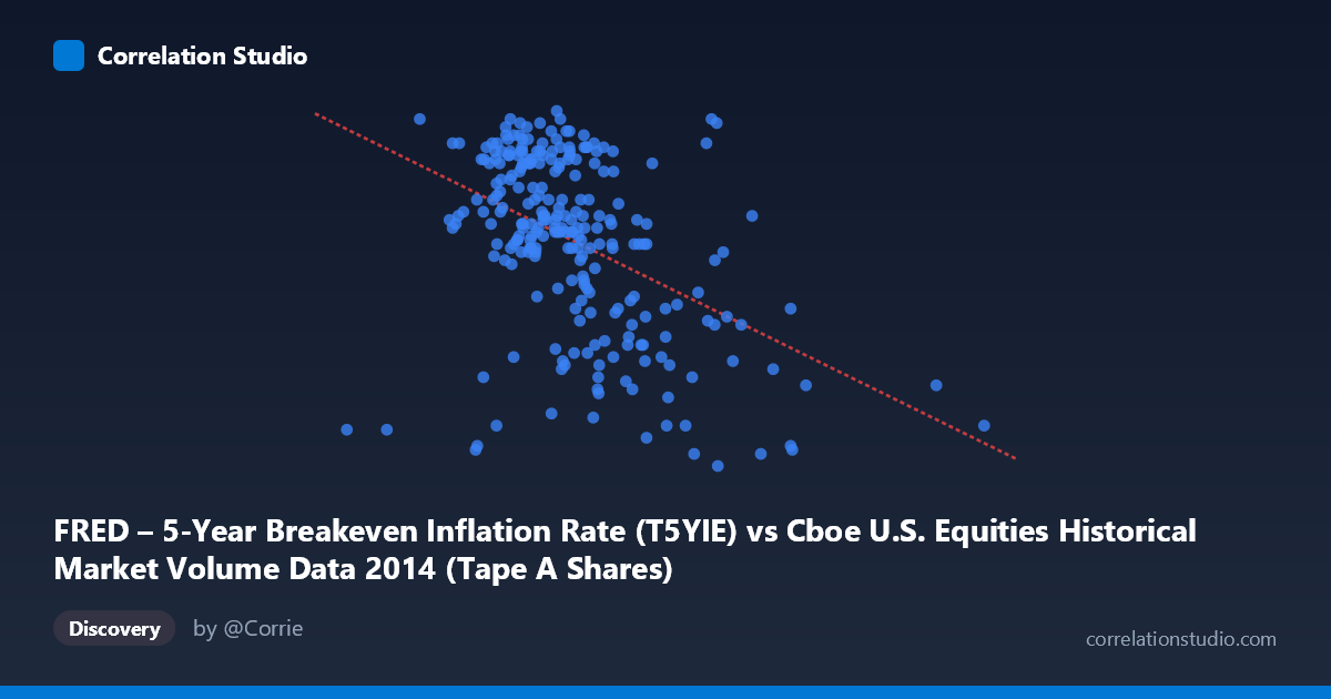
FRED – 5-Year Breakeven Inflation Rate (T5YIE) vs Cboe U.S. Equities Historical Market Volume Data 2014 (Tape A Shares)
- Pearson correlation (r)
- -0.449
- Spearman correlation
- -0.4398
- p-value
- 0
- Sample size (n)
- 250
- 95% confidence interval
- -0.5428 to -0.3441
- Granger causality
- None
- Granger optimal lag
- 1
AI analysis
Scatterplot Analysis: 5-Year Breakeven Inflation Rate vs. Cboe U.S. Equities Market Volume (2014)
Relationship Overview
The scatterplot reveals a negative relationship between Cboe U.S. equities market volume (x-axis) and the 5-year breakeven inflation rate (y-axis) across 2014 trading days. As daily equity trading volume increases, the breakeven inflation rate tends to decline. The linear regression equation (y = -2.145×10⁻⁹x + 2.22) captures this downward slope, suggesting that days with exceptionally high trading volume coincide with lower inflation expectations. This pattern is conceptually interesting — elevated equity market activity may reflect risk-off or volatility episodes during which inflation expectations compress — but the relationship is far from deterministic.
Correlation Strength and Statistical Significance
The Pearson correlation of r = -0.449 indicates a moderate negative association. However, the coefficient of determination r² = 0.2016 tells the more important story: only ~20% of the variance in the breakeven inflation rate is explained by trading volume, meaning roughly 80% of the variation remains attributable to other factors. The 95% confidence interval of [-0.543, -0.344] is meaningfully away from zero, and the p-value of 8.37×10⁻¹⁴ confirms this correlation is highly statistically significant given the sample of 250 paired observations drawn from a population of 3,686. Despite statistical significance, the Granger causality tests provide no support for temporal predictive directionality in either direction (X→Y: F=0.15, p=0.70; Y→X: F=0.001, p=0.97). This is a critical caveat: knowing yesterday's trading volume does not meaningfully help predict today's inflation expectations, and vice versa. The correlation reflects a contemporaneous association rather than a lead-lag dynamic.
Patterns, Clusters, and Outliers
Several notable features emerge from the sample points: - A visible cluster exists in the 180M–260M volume range where breakeven rates span widely from ~1.40 to ~2.05, indicating high variance at moderate volume levels and weakening the regression signal considerably - High-volume outliers (e.g., ~437M shares at 1.37, ~363M at 1.37, ~355M at 1.21) consistently appear at lower inflation expectations, anchoring the negative slope - Low-volume observations (e.g., ~124M at 1.26, ~143M at 2.03, ~175M at 1.22) are more dispersed but include some of the highest breakeven readings, consistent with the negative trend - There is a suggestion of non-linearity or heteroscedasticity: variance in the breakeven rate appears larger at mid-range volumes, potentially indicating that a simple linear model is not the best fit for this data
Confounding Factors and Interpretive Caveats
Several confounds complicate causal interpretation. First, both variables are time-indexed across 2014, meaning macro events — the Federal Reserve's QE tapering conclusion, geopolitical shocks (Ukraine, oil price decline in H2 2014), and broader risk sentiment shifts — likely drove simultaneous movements in both series, creating spurious or indirect correlation. The sharp oil price collapse in late 2014 is a particularly strong confounder, as it would have suppressed inflation expectations while potentially driving elevated equity market volume through volatility. Second, the breakeven rate is a forward-looking bond market signal while equity volume is a real-time activity measure; they operate in different markets with different participant bases. Third, the axes in the provided data summary appear to have dataset-column assignments swapped in the labels (the FRED breakeven rate is noted on both axes in different contexts), warranting verification of data pipeline integrity before drawing firm conclusions.
Actionable Insights and Further Investigation
Despite the absence of Granger causality, the moderate contemporaneous correlation warrants further exploration. Analysts should consider decomposing the time series to isolate whether the correlation holds in distinct market regimes (e.g., pre- vs. post-oil shock periods in 2014), which would help determine whether the relationship is driven by a specific macro episode rather than a structural link. Adding the VIX or realized volatility as a control variable could reveal whether elevated volume and depressed inflation expectations are both downstream of a common risk-aversion signal. A rolling correlation analysis across the year would show whether the relationship strengthened during the H2 2014 commodity-driven disinflationary episode. Finally, extending the analysis to multiple years would test whether this is a 2014-specific artifact or a more durable relationship worthy of incorporation into macro-trading or risk models.
X dataset: Cboe U.S. Equities Historical Market Volume Data 2014
Y dataset: FRED – 5-Year Breakeven Inflation Rate
Part of experiment: Daily - Cboe U.S. Equities Historical Market Volume Data 2014 vs FRED – 5-Year Breakeven Inflation Rate