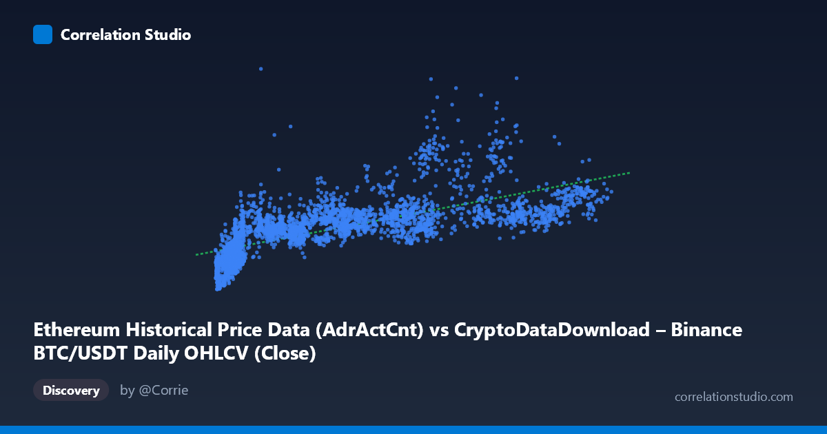
Ethereum Historical Price Data (AdrActCnt) vs CryptoDataDownload – Binance BTC/USDT Daily OHLCV (Close)

Pearson correlation (r): 0.6952
Spearman correlation: 0.8286
p-value: 0
Sample size (n): 3191
95% confidence interval: 0.6768 to 0.7127
Granger causality: None
Granger optimal lag: 10

AI analysis

Scatterplot Analysis: Ethereum Active Addresses vs. BTC/USDT Close Price

1. What the Visualization Reveals

The scatterplot shows a positive, moderately strong association between the X-variable (labeled as Ethereum active address count, though the axis title suggests some metadata confusion with BTC price data) and the Y-variable (BTC/USDT closing price). As X increases from roughly 3,000 to 125,000, Y trends upward from the 130K–1.5M range, but with substantial scatter around the fitted line — points fan out considerably, especially at mid-to-high X values, indicating that X alone does not tightly constrain Y.

2. Strength, Direction, and Statistical Confidence

The Pearson correlation of r = 0.695 indicates a moderately strong positive linear relationship, but r² = 0.483 means only about 48% of the variance in Y is explained by X — the majority of Y's variability (52%) is driven by other factors. The 95% CI [0.677, 0.713] is tight given the large sample (n=3,191), and the p-value of ~0 confirms the correlation is highly statistically significant — this is not due to chance. However, statistical significance with large n is expected even for modest effect sizes, so practical significance should be judged by r², not the p-value.

Critically, the Granger causality tests show no significant predictive direction in either direction (X→Y: p=0.717; Y→X: p=0.671). This means neither variable's historical values help forecast the other's future values at the tested lag (10 periods). This is an important caveat: despite the contemporaneous correlation, there's no evidence of a lead-lag temporal relationship — the co-movement may stem from both series responding to a common underlying driver (e.g., overall crypto market sentiment, liquidity cycles, or bull/bear regimes) rather than one causing the other.

3. Notable Patterns and Non-linearity

The data shows clear heteroscedasticity: variance in Y increases substantially as X grows, producing a cone/fan shape rather than a uniform linear band. At low X (<15,000), Y values cluster tightly between ~150K–500K. At higher X (60,000), Y ranges widely from ~500K to over 1.5M, suggesting the relationship may not be well-captured by a simple linear model. The note that Spearman ρ exceeds Pearson r supports this — a monotonic but non-linear (e.g., logarithmic or power-law) relationship likely fits better, which is common in financial/crypto series where percentage changes matter more than absolute levels. A few points (e.g., X≈65-90K with Y approaching 900K-1M) appear as high-leverage observations that could disproportionately affect the linear fit.

4. Confounding Factors and Caveats

- Metadata inconsistency: the axis labels reference both "Ethereum AdrActCnt" and "BTC/USDT Close" for X, creating ambiguity about what's actually being measured — this should be resolved before drawing conclusions. - Time-series autocorrelation: both series likely exhibit trends/momentum over the 2017–2026 span; naive Pearson/Spearman correlations on trending time series can produce spurious correlation from shared drift (e.g., overall crypto market growth) rather than genuine covariation. - Non-stationarity: crypto prices and on-chain metrics are typically non-stationary (unit-root behavior), which can inflate correlation estimates and invalidate standard significance tests unless differenced or detrended. - Market regime effects: bull/bear cycles (2017, 2021, 2024-25) could create clustered periods of high correlation alternating with decoupling, which a single aggregate r masks.

5. Suggested Next Steps

1. Clarify data provenance — confirm which variable is actually on each axis given the labeling conflict. 2. Detrend or difference both series (e.g., use daily/weekly % returns instead of levels) and recompute correlation to test whether the relationship holds after removing shared trend/non-stationarity. 3. Fit non-linear models (log-log, polynomial) given the Spearman-Pearson gap and visible heteroscedasticity; compare AIC/BIC against the linear fit. 4. Segment by market regime (bull vs. bear, or by year) to check if correlation strength is stable or concentrated in specific periods. 5. Given the null Granger result, avoid using one series to forecast the other; instead, investigate common macro drivers (BTC dominance, overall market cap, regulatory events) that might explain co-movement.

X dataset: CryptoDataDownload – Binance BTC/USDT Daily OHLCV

Y dataset: Ethereum Historical Price Data

Part of experiment: Bitcoin - CryptoDataDownload – Binance BTC/USDT Daily OHLCV vs Ethereum Historical Price Data