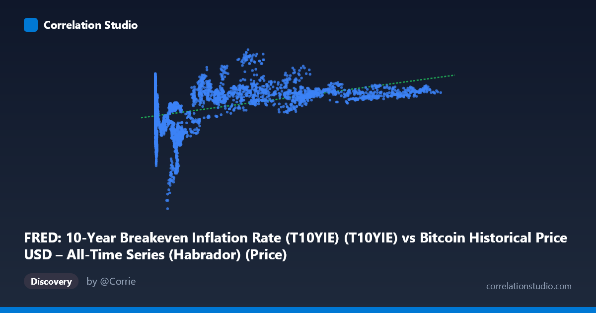
FRED: 10-Year Breakeven Inflation Rate (T10YIE) (T10YIE) vs Bitcoin Historical Price USD – All-Time Series (Habrador) (Price)
- Pearson correlation (r)
- 0.4417
- Spearman correlation
- 0.3367
- p-value
- 0
- Sample size (n)
- 4042
- 95% confidence interval
- 0.4165 to 0.4662
- Granger causality
- None
- Granger optimal lag
- 1
- Time coverage
- 2010-07-19 to 2026-09-15
- Recomputed on refreshed data
- 2026-10-24 (r was 0.4298)
AI analysis
Analysis: Bitcoin Price vs. 10-Year Breakeven Inflation Rate
1. Relationship Overview
Note first that the axis labels appear swapped relative to the data descriptions—the X-axis values (ranging from 0.05 to 124,720) are clearly Bitcoin prices in USD, while the Y-axis values (0.50 to 3.02) are clearly the T10YIE inflation expectation rate in percentage points. The analysis below treats the data according to its actual scale/units rather than the stated labels.
The scatterplot shows a positive but noisy relationship: as Bitcoin's price climbed from fractions of a cent through six figures, breakeven inflation expectations drifted upward from roughly 1.4–1.8% to a range clustering around 2.2–2.4%. The relationship is clearly non-linear in appearance—inflation expectations don't scale proportionally with price but rather seem to shift in regimes tied to Bitcoin's market cycle phases.
2. Strength, Direction, and Statistical Confidence
The correlation (r = 0.43) is moderate and positive, with r² indicating that only 18.5% of the variance in inflation expectations is explained by Bitcoin price (or vice versa)—leaving over 80% attributable to other factors. The 95% CI [0.404, 0.455] is tight, and the p-value of ~0 confirms this correlation is highly statistically significant and not due to chance, likely a function of the large sample size (n=3,946) rather than a strong practical effect. Critically, the Granger causality tests show no significant predictive direction in either direction (X→Y: p=0.46; Y→X: p=0.12). This means neither series reliably helps forecast the other's future values at a 1-period lag—the correlation is best understood as coincidental co-movement or a shared response to a common underlying driver (e.g., macroeconomic conditions, monetary policy, risk sentiment), not a causal or lead-lag relationship.
3. Notable Patterns and Features
The data reveals distinct clustering by price regime rather than a smooth linear trend: - Low-price era (X < 1,000): Inflation expectations are highly volatile, ranging from 1.4% to 2.5%, reflecting Bitcoin's early years spanning multiple macro regimes (2010s low-inflation period through 2020-21 COVID volatility). - Mid-range (X ~5,000–20,000): A notable dip cluster appears around 1.67–1.74%, corresponding likely to the 2018-2019 period of low inflation expectations. - High-price era (X 30,000): Inflation expectations compress into a narrower, elevated band (2.2–2.4%), coinciding with the 2021-2024 post-pandemic inflationary environment when Bitcoin also reached all-time highs.
This pattern suggests the correlation is driven largely by overlapping historical timing rather than a functional relationship—both series happened to rise together during the 2020-2024 macro era.
4. Confounding Factors and Caveats
This is a textbook case of spurious correlation risk via time-trend confounding. Both Bitcoin price and inflation expectations have exhibited long-term upward drift over the 2010-2026 window, and any two trending time series will show positive correlation even absent a causal link. Key confounders include: Federal Reserve policy (QE, rate decisions) affecting both risk assets and breakeven rates simultaneously; broad market liquidity/risk appetite cycles; Bitcoin's idiosyncratic adoption-driven price appreciation unrelated to macro variables; and the non-stationarity of both series (prices and rates rarely revert to a stable mean, violating assumptions of simple Pearson correlation).
5. Recommendations for Further Investigation
- Detrend or difference both series (e.g., use log returns for BTC and first-differences for T10YIE) and recompute correlation—this will likely reveal a much weaker or near-zero relationship, testing whether the raw correlation is purely trend-driven. - Segment by macro regime (pre-2020 vs. post-2020) to check if the relationship is regime-dependent rather than universal. - Test additional lags in Granger causality (beyond lag=1) and consider VAR models with control variables (real rates, DXY, equity indices) to isolate any genuine predictive content. - Treat this correlation as descriptive, not predictive or causal—given the weak r², lack of Granger causality, and plausible trend confounding, this relationship should not be used for trading signals or forecasting without substantially more rigorous econometric treatment (cointegration testing, stationarity checks).
X dataset: Bitcoin Historical Price USD – All-Time Series (Habrador)
Y dataset: FRED: 10-Year Breakeven Inflation Rate (T10YIE)
Part of experiment: Bitcoin - Bitcoin Historical Price USD – All-Time Series (Habrador) vs FRED: 10-Year Breakeven Inflation Rate (T10YIE)