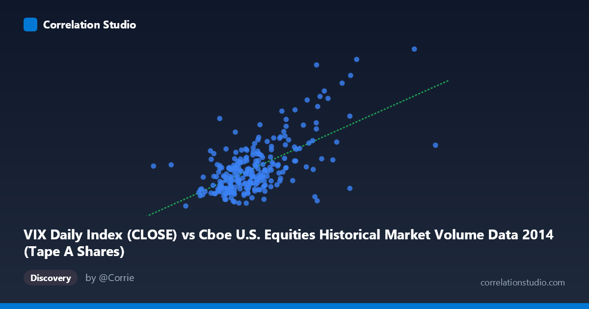
VIX Daily Index (CLOSE) vs Cboe U.S. Equities Historical Market Volume Data 2014 (Tape A Shares)

Pearson correlation (r): 0.62
Spearman correlation: 0.5071
p-value: 0
Sample size (n): 252
95% confidence interval: 0.5376 to 0.6906
Granger causality: None
Granger optimal lag: 1

AI analysis

Scatterplot Analysis: VIX vs. Tape A Share Volume (2014)

Relationship Overview

The scatterplot reveals a moderate positive relationship between the CBOE Volatility Index (VIX) and Tape A share volume in U.S. equity markets during 2014. As VIX levels rise — indicating greater expected market volatility — trading volume in Tape A shares tends to increase correspondingly. This aligns intuitively with market microstructure theory: periods of heightened uncertainty and fear typically drive elevated trading activity as investors rebalance, hedge, or exit positions. The linear regression equation (y = 3.55×10⁻⁸x + 5.997) captures this upward slope, though the wide scatter around the regression line immediately signals that volume is far from fully determined by VIX alone.

Correlation Strength and Statistical Framing

The correlation coefficient of r = 0.620 indicates a moderate-to-strong positive association, but the coefficient of determination (r² = 0.384) is the more sobering figure: only 38.4% of the variance in Tape A share volume is explained by VIX. That leaves roughly 62% of volume variation attributable to other factors entirely. The 95% confidence interval for r spans [0.538, 0.691], which is meaningfully wide but excludes zero comfortably, and the p-value of effectively 0 across a sample of n = 252 confirms this relationship is not a statistical artifact. Critically, however, the Granger causality tests find no significant predictive directionality in either direction (X→Y: F = 1.75, p = 0.187; Y→X: F = 0.43, p = 0.511). This means that while VIX and volume move together contemporaneously, neither variable reliably predicts the other with a one-period lag — a meaningful distinction for any practical forecasting application.

Notable Patterns, Clusters, and Outliers

Several structural features stand out in the data. The bulk of observations cluster in a dense core roughly between VIX values of 11–17 and volume levels of 12–16 billion shares, reflecting the prolonged low-volatility environment that characterized much of 2014. Above this core, a distinct upper-right cluster of points — visible in sample observations like (362,472,905; 25.20) and (354,712,059; 23.57) — represents high-VIX, high-volume episodes, likely corresponding to the October 2014 market correction. These points exert considerable leverage on the regression slope and may be driving much of the observed correlation. Conversely, there is a notable outlier near (311,714,842; 10.85) — unusually high volume paired with a very low VIX — which defies the general trend and warrants separate investigation. This heteroscedasticity (wider spread at higher VIX values) suggests the linear model's assumptions may not fully hold across the data range.

Confounding Factors and Caveats

Several important caveats temper interpretation. First, seasonal and calendar effects in 2014 likely co-drive both variables simultaneously — end-of-quarter rebalancing, options expiration dates, and macroeconomic announcements elevate both volatility and volume independently, creating spurious correlation. Second, the relationship may be non-linear: volume may respond asymmetrically to VIX spikes versus gradual VIX drift, which a linear model cannot capture. Third, Tape A specifically captures NYSE-listed securities; VIX is derived from S&P 500 index options, so the universe mismatch introduces noise. Fourth, the dataset covers only a single calendar year (2014), a period of unusually compressed volatility for much of the year followed by a sharp spike — this structural regime change means findings may not generalize to other market environments.

Actionable Insights and Further Investigation

Practitioners and researchers should pursue several follow-up directions. First, segmenting the data by volatility regime (e.g., VIX < 15 vs. VIX ≥ 15) would reveal whether the correlation holds uniformly or is concentrated in high-stress periods. Second, testing non-linear models (polynomial, piecewise, or log-transformed) may substantially improve fit given the visible heteroscedasticity. Third, extending the Granger causality analysis to longer lags (beyond 1 period) could uncover delayed predictive relationships that a single-lag test misses. Fourth, incorporating additional covariates — such as options open interest, bid-ask spreads, or macroeconomic surprise indices — would help isolate the independent contribution of VIX to volume variation. Finally, replicating this analysis across multiple years would test whether the observed r = 0.62 is a stable structural feature of U.S. equity markets or an artifact of 2014's particular volatility narrative.

X dataset: Cboe U.S. Equities Historical Market Volume Data 2014

Y dataset: VIX Daily Index

Part of experiment: Daily - Cboe U.S. Equities Historical Market Volume Data 2014 vs VIX Daily Index