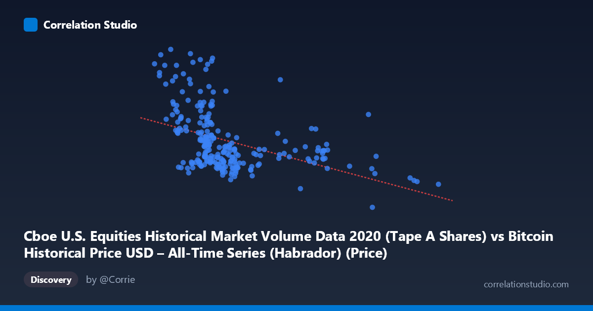
Cboe U.S. Equities Historical Market Volume Data 2020 (Tape A Shares) vs Bitcoin Historical Price USD – All-Time Series (Habrador) (Price)
- Pearson correlation (r)
- -0.4391
- Spearman correlation
- -0.5188
- p-value
- 0
- Sample size (n)
- 253
- 95% confidence interval
- -0.5335 to -0.3339
- Granger causality
- None
- Granger optimal lag
- 10
- Time coverage
- 2020-01-02 to 2020-12-31
- Recomputed on refreshed data
- 2026-10-24 (r was -0.4391)
AI analysis
Analysis: Cboe Equities Volume vs. Bitcoin Price (2020)
1. What the Visualization Reveals
The scatterplot shows a moderate negative relationship between U.S. equities market volume (X) and Bitcoin price (Y) across 2020. The data forms a dense cluster in the lower-left region (X: 7,000–12,000; Y: $200M–$350M scale, noting these appear to be volume/notional figures in the hundreds of millions), with a long right-tail of higher-X observations extending to ~28,000+ that mostly correspond to lower Y-values. Several high-Y outliers (400M–565M) appear at low-to-mid X values, creating a visually scattered, funnel-like pattern rather than a tight linear band.
2. Strength, Direction, and Statistical Confidence
The correlation coefficient (r = -0.439) indicates a weak-to-moderate negative relationship. The r² of 0.193 means only 19.3% of the variance in Bitcoin price is explained by equities volume — leaving over 80% of price movement attributable to other factors. The 95% CI [-0.53, -0.33] is reasonably tight and excludes zero, and the p-value (2.4e-13) confirms this correlation is highly unlikely due to chance. However, statistical significance ≠ practical strength — this is a real but modest association, not a reliable predictive relationship.
Critically, the Granger causality tests show no significant predictive direction in either direction (X→Y: p=0.93; Y→X: p=0.72). This means that despite the contemporaneous negative correlation, past values of one series do not help forecast future values of the other. This strongly suggests the correlation is not causal and may instead reflect both series independently trending over 2020 (e.g., both reacting to the same macro shocks like the COVID crash) rather than one driving the other.
3. Notable Patterns and Outliers
- Clustering: The bulk of observations sit in a tight X-band (7,000–12,000), suggesting this is the "normal" trading volume regime for most of 2020. - High-Y outliers at low X: Points like (9811, 540M), (8785, 536M), and (5800, 519M) suggest a period (likely the March 2020 COVID crash or subsequent volatility spike) where Bitcoin-correlated prices surged while equity volume was only moderate — an unusual regime. - Low-Y, high-X tail: Points beyond X=15,000 (e.g., 19464, 23177, 23433) consistently show suppressed Y-values (~200-330M), hinting at a distinct market regime (possibly later 2020) where high equity volume coincided with more subdued price action. - The pattern is non-linear-looking, more consistent with two or three distinct regimes/clusters than a single linear trend, which likely deflates the linear r² and may better fit a piecewise or regime-switching model.
4. Confounding Factors and Caveats
- Time-series autocorrelation: Both series are daily 2020 data and likely highly autocorrelated; naive Pearson correlation on trending time series can produce spurious relationships (classic "trending series" confound). - Common external driver: 2020 was dominated by COVID-19 market shocks — both equities volume and Bitcoin price likely responded to the same volatility event independently, not to each other. - Mismatched labeling: The axis descriptions are oddly cross-labeled (X described as volume data, but tied to a "Price" dataset name, and Y described as Bitcoin price yet under a "volume" dataset title) — this warrants verification of correct variable assignment before drawing conclusions. - Non-stationarity: Neither series likely has constant mean/variance across 2020, which can distort both correlation and Granger test validity.
5. Suggested Next Steps
- Detrend or difference both series before re-testing correlation/Granger causality to remove spurious trend-driven association. - Segment analysis by regime (pre-crash, crash, recovery, year-end) to see if the negative correlation holds within each period or is purely a between-regime artifact. - Introduce a third-variable control (e.g., VIX, USD index) to test if a common shock variable better explains the joint movement. - Verify axis/data labeling to ensure the volume and price fields are correctly assigned before further modeling. - Given the lack of Granger causality, treat this relationship as descriptive/correlational only — not suitable for building a predictive trading signal in its current form.
X dataset: Bitcoin Historical Price USD – All-Time Series (Habrador)
Y dataset: Cboe U.S. Equities Historical Market Volume Data 2020
Part of experiment: Bitcoin - Bitcoin Historical Price USD – All-Time Series (Habrador) vs Cboe U.S. Equities Historical Market Volume Data 2020