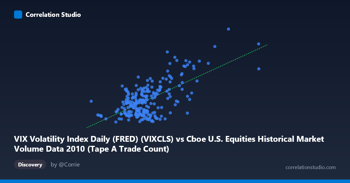
VIX Volatility Index Daily (FRED) (VIXCLS) vs Cboe U.S. Equities Historical Market Volume Data 2010 (Tape A Trade Count)
- Pearson correlation (r)
- 0.6492
- Spearman correlation
- 0.4347
- p-value
- 0
- Sample size (n)
- 252
- 95% confidence interval
- 0.5714 to 0.7154
- Granger causality
- Y → X
- Granger optimal lag
- 1
AI analysis
Analysis: VIX Volatility Index vs. Cboe Tape A Trade Count (2010)
Relationship Overview The scatterplot reveals a moderate-to-strong positive relationship between the VIX Volatility Index and Cboe Tape A Trade Count across 252 trading days in 2010. As the VIX rises — indicating greater market fear and implied volatility — the number of Tape A trades increases correspondingly. This is intuitively coherent: periods of market stress and uncertainty typically drive heightened trading activity as investors rebalance portfolios, hedge positions, or react to news. The linear regression equation (y = 8.84×10⁻⁶x + 10.91) confirms this positive slope, though the intercept suggests a meaningful baseline level of trade activity even during calm market conditions.
Correlation Strength and Causality The correlation coefficient of r = 0.649 indicates a moderate-to-strong positive association, but the more informative metric is r² = 0.421 — meaning roughly 42% of the variance in trade count is explained by VIX levels, while the remaining 58% is driven by other factors entirely. The 95% confidence interval [0.571, 0.715] is reassuringly tight and does not approach zero, and the p-value of effectively 0 confirms this is not a chance finding across the n = 252 sample drawn from a population of N = 3,302. Critically, the Granger causality results suggest a unidirectional temporal relationship: VIX Granger-causes trade count (Y→X: F = 7.99, p = 0.005), while the reverse direction (X→Y) fails to reach significance (F = 3.71, p = 0.055). This implies that rising VIX levels today are predictive of increased trading volume the following day, a practically important asymmetry — volatility sentiment leads volume, not the other way around.
Notable Patterns and Outliers Several features stand out in the data. The bulk of observations cluster in the lower-left region — VIX values roughly below 25 and trade counts below ~25 million — reflecting the relatively stable first half of 2010. However, a distinct upper-right cluster is visible, corresponding to periods of elevated VIX (30–45+) and substantially higher trade counts, likely coinciding with the May 2010 Flash Crash and subsequent European sovereign debt crisis anxiety. Points such as (3,216,587, 40.95) and (2,474,888, 40.10) represent clear high-leverage outliers that could disproportionately influence the regression slope. There also appears to be increased variance (heteroscedasticity) at higher VIX values — the spread of trade counts widens as volatility rises — suggesting the linear model may underfit the relationship at market extremes.
Confounding Factors and Caveats Several important caveats apply. First, 2010 was a structurally unusual year containing the May 6 Flash Crash, which likely creates an artifact cluster inflating both VIX and volume simultaneously — making the correlation partly an artifact of a single extreme event. Second, Tape A trade count reflects only NYSE-listed securities, not the full market, introducing a selection bias. Third, algorithmic and high-frequency trading activity in 2010 was accelerating rapidly, meaning trade count is not equivalent to genuine investor participation — machines generate elevated counts during volatility independently of human sentiment. Fourth, day-of-week effects, options expiration cycles, and macroeconomic data release schedules all co-vary with both VIX and trading activity, representing unmeasured confounders that could inflate the apparent relationship.
Actionable Insights and Further Investigation The Granger causality finding — that VIX predicts next-day trade count with a 1-period lag — has practical implications for market microstructure forecasting and exchange capacity planning. Exchanges and brokers could use VIX thresholds as leading indicators for expected system load. For researchers, priority next steps should include: (1) testing whether this relationship holds across multiple years (2008 crisis vs. low-volatility regimes like 2017) to assess structural stability; (2) applying a log transformation to both variables to address heteroscedasticity and potential power-law dynamics; (3) controlling for the Flash Crash period specifically to isolate its leverage on the regression; and (4) expanding to Tape B and C data to test whether the VIX-volume relationship is consistent across exchange types. A non-linear or piecewise regression model with a VIX breakpoint around 25–30 may also substantially improve explanatory power beyond the current 42%.
X dataset: Cboe U.S. Equities Historical Market Volume Data 2010
Y dataset: VIX Volatility Index Daily (FRED)
Part of experiment: Daily - Cboe U.S. Equities Historical Market Volume Data 2010 vs VIX Volatility Index Daily (FRED)