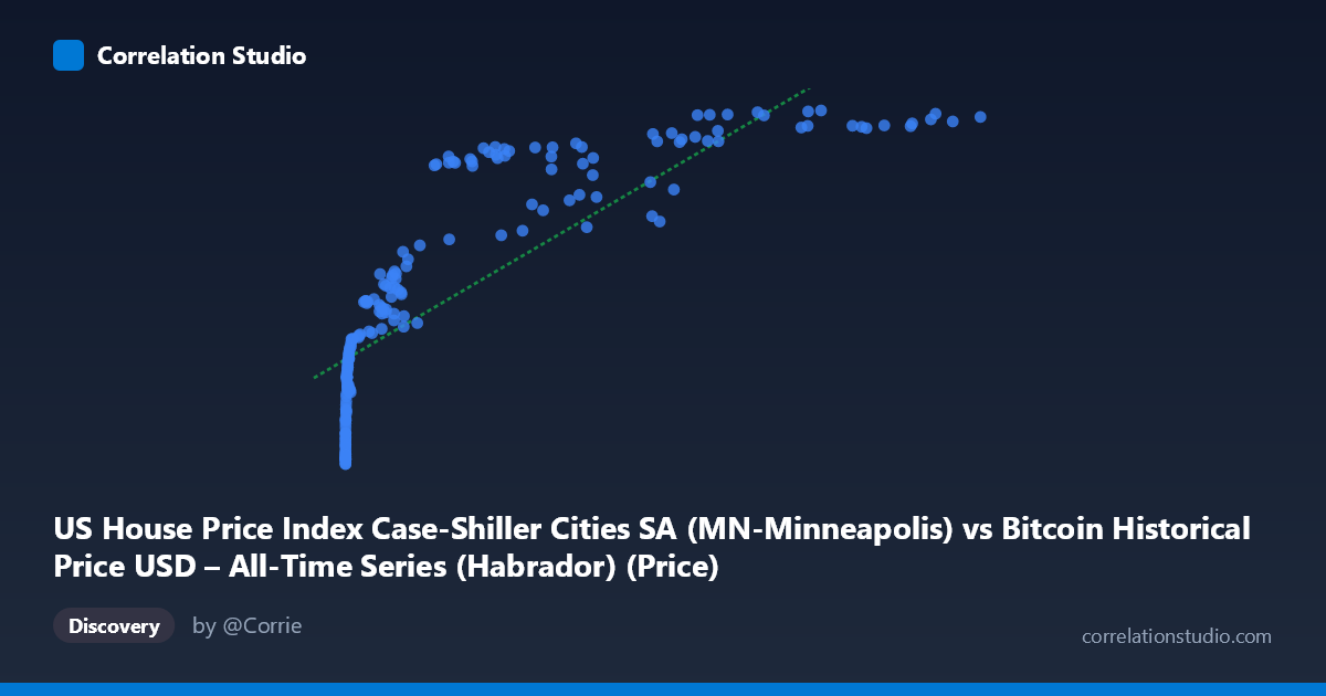
US House Price Index Case-Shiller Cities SA (MN-Minneapolis) vs Bitcoin Historical Price USD – All-Time Series (Habrador) (Price)
- Pearson correlation (r)
- 0.8166
- Spearman correlation
- 0.9707
- p-value
- 0
- Sample size (n)
- 187
- 95% confidence interval
- 0.7624 to 0.8594
- Granger causality
- None
- Granger optimal lag
- 1
AI analysis
Analysis: Bitcoin Price vs. Minneapolis Case-Shiller Home Price Index
1. What the Visualization Reveals
The scatterplot shows a strong positive association between Bitcoin's historical USD price (X-axis) and the Minneapolis Case-Shiller Home Price Index (Y-axis). The relationship is clearly non-linear: Y rises steeply as X moves from near-zero to roughly 1,000, then the curve flattens considerably as X extends into the tens of thousands and beyond (e.g., HPI moves from ~110 to ~160 as BTC goes from $0.06 to ~$1,000, but only from ~200 to ~250 as BTC goes from $20,000 to $118,000). This concave, logarithmic-like shape is consistent with the note that Spearman's ρ exceeds Pearson's r — a log or power transformation of X would likely produce a tighter fit than the linear model.
2. Strength, Direction, and Statistical Confidence
The Pearson correlation (r = 0.817, r² = 0.667) indicates a strong positive linear relationship, with the linear model explaining about 67% of the variance in the home price index. The 95% CI [0.762, 0.859] is fairly tight and excludes zero, and the p-value is effectively 0, so the correlation is highly unlikely to be a statistical fluke given this sample. However, correlation here should not be read as causation: the Granger causality tests show no significant predictive direction in either direction (BTC→HPI: p=0.34; HPI→BTC: p=0.11). This means neither series reliably helps forecast the other's future values given its own past — the strong contemporaneous correlation is likely driven by both variables trending upward over the same calendar period rather than one series mechanically driving the other.
3. Notable Patterns and Outliers
- Compression at low X: The vast majority of low-value BTC prices (X < 1,000) cluster tightly with HPI values between ~110–170, showing rapid index growth per unit of early BTC price change. - Flattening at high X: Once BTC exceeds ~$20,000, HPI growth decelerates and hovers in a narrow 200–250 band, despite BTC ranging from $20K to nearly $119K — a 6x range in X mapping to only a 25% range in Y. - Some scatter/noise at high X: Points like (29,111.52, 200.78) and (45,092.81, 203.96) sit noticeably below the general trend at similar X values compared to neighbors like (44,354.64, 229.11), suggesting real estate cycles (seasonal dips, 2022–2023 rate-driven corrections) introduce vertical scatter not explained by BTC price alone. - No extreme outliers distort the fit; the non-linearity is the dominant visual feature rather than isolated anomalies.
4. Confounding Factors and Caveats
This is a classic spurious/coincidental trend correlation: both Bitcoin price and home price indices have broadly risen over 2010–2026, driven by shared macro factors (loose monetary policy, low interest rates in 2010s, inflation post-2020, general asset price appreciation) rather than any direct economic link between Bitcoin markets and Minneapolis housing. Time itself is a likely lurking confounder — both series are non-stationary and trending, which inflates Pearson correlation even absent a causal mechanism (a well-known issue with naive correlation of two trending time series). The lack of Granger causality reinforces that this is not a predictive relationship. Additionally, Bitcoin's extreme scale (spanning $0.06 to $118,670, 6 orders of magnitude) versus HPI's modest range (110–250) makes the linear r/r² somewhat misleading as a "fit" metric.
5. Suggested Next Steps
- Detrend or difference both series (e.g., use month-over-month % changes rather than levels) and recompute correlation to test whether the relationship survives after removing shared time trends — this is critical given the non-stationarity concern. - Fit a log-linear model (log(X) vs. Y) given the Spearman/Pearson divergence; this should improve R² and better reflect the true functional form. - Compare against a neutral time-only control, such as correlating each series independently with a simple time index, to gauge how much of the r=0.82 is just "both go up over time." - Treat this correlation as descriptive/coincidental rather than a basis for trading or economic strategy — the Granger results are the strongest evidence against using one series to forecast the other.
X dataset: Bitcoin Historical Price USD – All-Time Series (Habrador)
Y dataset: US House Price Index Case-Shiller Cities SA
Part of experiment: Bitcoin - Bitcoin Historical Price USD – All-Time Series (Habrador) vs US House Price Index Case-Shiller Cities SA