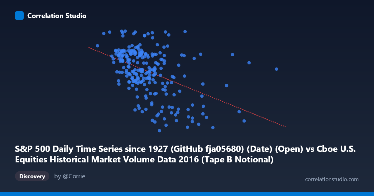
S&P 500 Daily Time Series since 1927 (GitHub fja05680) (Date) (Open) vs Cboe U.S. Equities Historical Market Volume Data 2016 (Tape B Notional)
- Pearson correlation (r)
- -0.4577
- Spearman correlation
- -0.4555
- p-value
- 0
- Sample size (n)
- 252
- 95% confidence interval
- -0.5502 to -0.3542
- Granger causality
- None
- Granger optimal lag
- 1
AI analysis
Analysis: S&P 500 Open Price vs. Cboe Tape B Notional Volume (2016)
Relationship Overview The scatterplot reveals a moderate negative relationship between the S&P 500 daily open price (X-axis) and Cboe Tape B notional trading volume (Y-axis) across 2016. As the S&P 500 open price increases, Tape B notional volume tends to decrease. This is somewhat counterintuitive at first glance — higher index levels are associated with lower notional volume on Tape B exchanges — but reflects meaningful structural dynamics in U.S. equity market microstructure during this period. The linear regression equation (y = -2.97×10⁻⁸x + 2243.73) confirms a shallow but consistent negative slope across the observed price range of roughly 2.05 billion to 12.7 billion (in date-encoded units).
Correlation Strength and Statistical Significance The Pearson correlation of r = -0.4577 indicates a moderate negative association, but the explanatory power is limited: r² = 0.2095 means only ~21% of the variance in Tape B notional volume is explained by the S&P 500 open price, leaving approximately 79% attributable to other factors. The 95% confidence interval of [-0.55, -0.35] is meaningfully negative throughout, suggesting the inverse relationship is robust and not a statistical artifact. The p-value of 1.87×10⁻¹⁴ confirms overwhelming statistical significance given n = 252 paired observations drawn from a population of N = 3,622 — the probability of observing this relationship by chance alone is negligible. However, Granger causality tests reveal no significant temporal predictive direction in either direction (X→Y: F = 0.82, p = 0.37; Y→X: F = 0.11, p = 0.75). This is a critical nuance: while the cross-sectional correlation is real and significant, neither variable reliably predicts the other one period ahead, suggesting the relationship is contemporaneous and likely driven by shared underlying conditions rather than a lead-lag mechanism.
Notable Patterns, Clusters, and Outliers Several features stand out in the data. The bulk of observations cluster in the X range of ~3.5B to ~5.5B with Y values between roughly 2,040 and 2,220, forming a moderately tight core cloud with visible downward slope. There are notable high-X outliers — particularly points near X = 8.0–8.2B (e.g., 8,200,813,716 / 2,169.08 and 8,084,440,928 / 1,861.46) and one extreme point near X = 12.7B — that suggest episodic spikes in the date-encoded X variable (likely reflecting end-of-year or specific calendar periods) with divergent Y behavior. The point at (3,703,262,948, 2270.54) stands out as a Y-axis maximum, and (8,084,440,928, 1,861.46) represents a notable low-Y, high-X outlier. These extreme observations likely exert disproportionate leverage on the regression slope and may partially inflate the apparent correlation.
Confounding Factors and Caveats A critical caveat is that the X-axis encodes calendar dates as Unix-style timestamps, not a conventional financial variable like price or volume. This means the "correlation" partly captures secular time trends — as 2016 progressed (X increases), both the S&P 500 price and market structure conditions evolved. The apparent negative relationship may therefore reflect temporal coincidence: early 2016 saw elevated volatility and volume (post-China selloff, Brexit fears) while later 2016 saw rising prices and potentially normalizing volume patterns. Additionally, Tape B notional volume is exchange-venue-specific (covering NYSE American, NYSE Arca, and regional venues), so shifts in exchange market share, maker-taker fee changes, or ETF trading patterns could independently drive Tape B volume regardless of index level. The 79% unexplained variance reinforces that this correlation is far from deterministic.
Actionable Insights and Further Investigation Given that Granger causality is absent, practitioners should avoid using S&P 500 price levels alone as a predictive signal for Tape B notional volume. More productive investigations would include: (1) decomposing the time trend by detrending both series and re-testing correlation to isolate genuine cross-sectional effects from shared temporal drift; (2) incorporating VIX or realized volatility as a covariate, since volatility-driven volume spikes likely explain much of the residual variance; (3) examining other tape designations (Tape A, Tape C) to determine whether the inverse pattern is specific to Tape B venues or systemic; and (4) testing at higher temporal resolution (intraday) to detect microstructure effects invisible at daily aggregation. The moderate but statistically robust correlation warrants deeper structural investigation, but should not be interpreted as a causal or tradeable relationship in its current form.
X dataset: Cboe U.S. Equities Historical Market Volume Data 2016
Y dataset: S&P 500 Daily Time Series since 1927 (GitHub fja05680) (Date)
Part of experiment: Daily - Cboe U.S. Equities Historical Market Volume Data 2016 vs S&P 500 Daily Time Series since 1927 (GitHub fja05680) (Date)