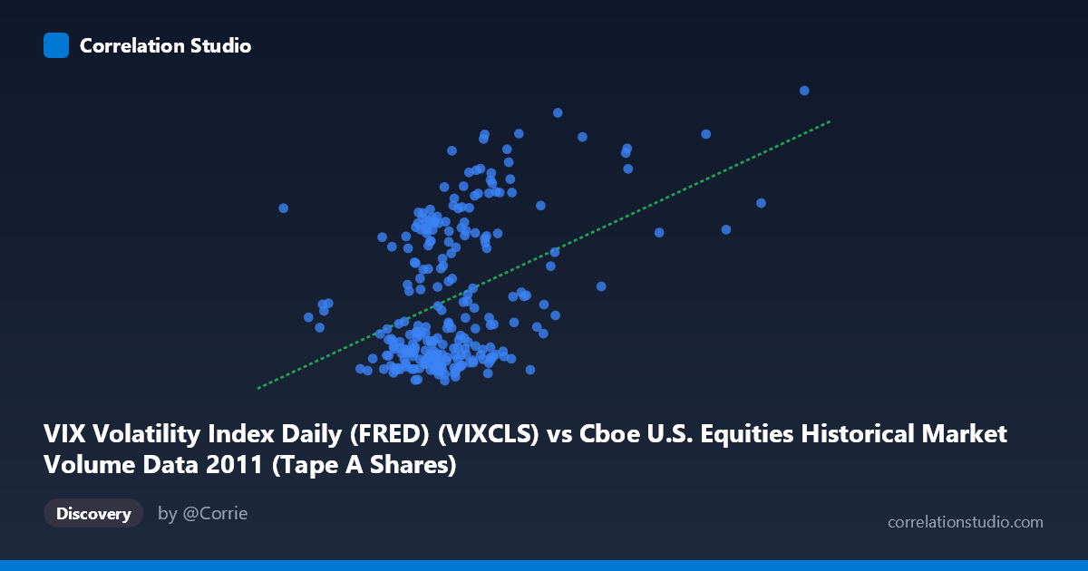
VIX Volatility Index Daily (FRED) (VIXCLS) vs Cboe U.S. Equities Historical Market Volume Data 2011 (Tape A Shares)
- Pearson correlation (r)
- 0.4187
- Spearman correlation
- 0.3334
- p-value
- 0
- Sample size (n)
- 252
- 95% confidence interval
- 0.3113 to 0.5156
- Granger causality
- None
- Granger optimal lag
- 1
AI analysis
Analysis: VIX Volatility Index vs. Cboe U.S. Equities Market Volume (Tape A Shares) — 2011
1. Overall Relationship Revealed
The scatterplot reveals a positive but notably scattered relationship between daily U.S. equities market volume (X-axis, measured in notional value) and the VIX Volatility Index (Y-axis). The linear regression equation (y = 5.07744E-08x + 9.50) confirms a positive slope, meaning that as trading volume increases, VIX tends to rise as well. This is intuitively consistent with market microstructure theory: periods of elevated fear and uncertainty tend to drive both higher implied volatility (VIX) and heavier trading activity as investors reposition portfolios. However, the wide dispersion around the regression line makes clear that volume alone is far from a reliable predictor of VIX levels.
2. Correlation Strength, Direction, and Temporal Causality
The Pearson correlation of r = 0.4187 indicates a moderate positive association, but the explanatory power is modest: r² = 0.1754 means only ~17.5% of the variance in VIX is explained by trading volume, leaving roughly 82.5% attributable to other factors. The 95% confidence interval of [0.3113, 0.5156] is meaningfully bounded away from zero, and the p-value of 4.04E-12 confirms this correlation is highly statistically significant — not a sampling artifact — given the paired sample of n = 252 drawn from a population of N = 3,780 observations. However, statistical significance should not be conflated with practical predictive power; the wide CI spread (~0.2 units) reflects genuine uncertainty in the precise magnitude of the relationship. Critically, the Granger causality tests show no significant predictive directionality in either direction (X→Y: F = 0.0716, p = 0.79; Y→X: F = 0.0013, p = 0.97). This means that past values of volume do not help predict future VIX, and vice versa — the two series move together contemporaneously but neither leads the other temporally, which substantially limits actionable trading signals derived from this relationship alone.
3. Notable Patterns, Clusters, and Outliers
Several structural features are visible in the data: - A dense core cluster sits in the volume range of roughly 220–340 million (X) and VIX range of 15–25, representing typical low-to-moderate volatility trading days that dominate the 2011 calendar - A high-VIX arm extends upward (VIX 30–48) at moderate-to-high volume levels, corresponding to identifiable stress episodes in 2011 — most notably the August 2011 U.S. debt ceiling crisis and S&P sovereign downgrade, which drove VIX briefly above 45 - High-volume, low-VIX days are also present (e.g., volume ~450–660 million with VIX near 25), suggesting that mechanically elevated volume can occur without fear-driven volatility, perhaps reflecting index rebalancing or expiration-related flows - Sample points like (474,714,411, 39.00) and (446,339,770, 25.46) illustrate this divergence — similar high-volume days can coincide with very different VIX readings, underscoring the heteroscedastic spread that widens at higher volume levels
4. Confounding Factors and Interpretive Caveats
Several important caveats temper interpretation: - Temporal confounding: 2011 was an unusually eventful year (Arab Spring, Eurozone sovereign debt crisis, U.S. downgrade), meaning stress clustering rather than a structural volume-VIX relationship may be driving the correlation - Bidirectional contemporaneous causation: High VIX may cause high volume (fear-driven selling) and high volume may signal uncertainty that feeds VIX — these cannot be separated without intraday data - Tape A specificity: Tape A covers NYSE-listed securities only; the relationship may differ for Tape B (NYSE American) or Tape C (Nasdaq), limiting generalizability - Non-linearity: The scatter suggests the relationship may be stronger at extreme values (tail events) and weaker during calm periods — a linear model may underfit the true functional form - Regime dependence: The correlation likely varies significantly across different volatility regimes; pooling all 252 days obscures whether the relationship holds in both calm and stressed market conditions
5. Actionable Insights and Further Investigation
Despite the Granger causality null result, the moderate contemporaneous correlation offers several directions worth pursuing: - Regime-segmented analysis: Split the dataset into low-VIX (< 20), moderate (20–30), and high-VIX ( 30) regimes to test whether the volume-VIX relationship is driven disproportionately by tail-stress periods - Non-linear modeling: Fit a log-log or quadratic model to assess whether the relationship is better captured by a power law, which would be consistent with microstructure literature on volume-volatility dynamics - Lag structure expansion: The Granger test used only lag = 1; testing lags of 2–5 days may reveal delayed predictive relationships, especially given that volatility clustering (GARCH effects) is well-documented in VIX - Cross-year validation: Replicate this analysis across 2008–2010 and 2012–2015 to determine whether the r = 0.42 finding is stable or specific to 2011's unique macro environment - Multivariate modeling: Introduce additional covariates (S&P 500 returns, put/call ratio, credit spreads) to decompose the 82.5% unexplained variance and build a more actionable predictive framework for VIX conditional on volume signals
X dataset: Cboe U.S. Equities Historical Market Volume Data 2011
Y dataset: VIX Volatility Index Daily (FRED)
Part of experiment: Daily - Cboe U.S. Equities Historical Market Volume Data 2011 vs VIX Volatility Index Daily (FRED)