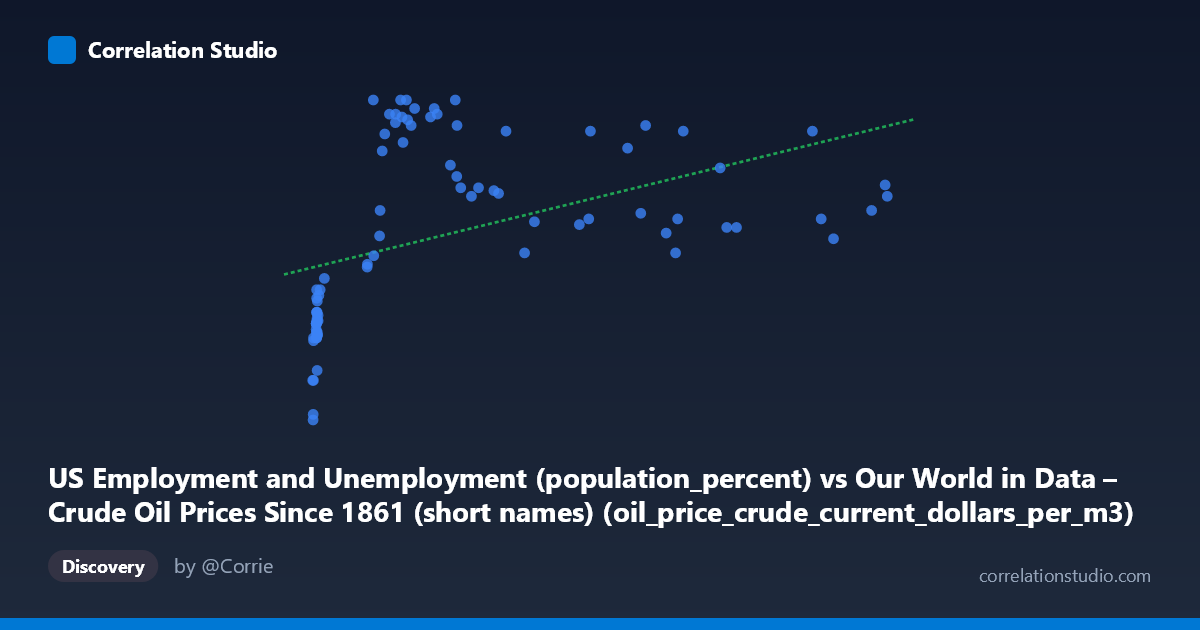
US Employment and Unemployment (population_percent) vs Our World in Data – Crude Oil Prices Since 1861 (short names) (oil_price_crude_current_dollars_per_m3)
- Pearson correlation (r)
- 0.4474
- Spearman correlation
- 0.689
- p-value
- 0.000018
- Sample size (n)
- 85
- 95% confidence interval
- 0.2589 to 0.603
- Granger causality
- None
- Granger optimal lag
- 1
AI analysis
Analysis: Crude Oil Prices vs. US Unemployment Rate (1941–2024)
1. What the Visualization Reveals
The scatterplot displays a modest positive relationship between crude oil prices (in current dollars per cubic meter) on the X-axis and the US employment/unemployment population percentage on the Y-axis, spanning over eight decades of annual data. The overall pattern shows that as oil prices have risen historically, the unemployment-related metric has trended slightly upward. However, the data is clearly not distributed uniformly — there is a pronounced clustering of points at very low X-values (below ~50), and a more dispersed spread across higher price ranges, suggesting the relationship is far from simple or linear.
2. Correlation Strength, Direction, and Causality
The Pearson correlation of r = 0.452 indicates a moderate positive association, but the explanatory power is limited: R² = 0.204, meaning crude oil prices account for only about 20% of the variance in the unemployment metric. The remaining 80% is driven by other factors entirely. The 95% confidence interval for r spans [0.263, 0.608], which is meaningfully wide, reflecting genuine uncertainty about the true population relationship. The p-value of 1.58 × 10⁻⁵ confirms the correlation is statistically significant and unlikely due to chance. Crucially, however, the Granger causality tests found no significant predictive direction in either direction at the tested lag — neither does oil price reliably predict future unemployment changes (F = 0.43, p = 0.52), nor does unemployment predict future oil prices (F = 3.30, p = 0.073). This means that while the two variables move together historically, neither demonstrably leads the other in a temporally predictive sense.
3. Notable Patterns, Clusters, and Non-Linearity
Several structural features stand out. First, there is a dense cluster of points near X = 7–15 with Y-values concentrated around 57–60.5, representing the low-price, mid-20th century era when oil was cheap and unemployment figures were in a distinct regime. Second, a separate cluster emerges at X = 70–200 with Y-values mostly between 62–67, suggesting a step-change rather than a smooth progression. Third, the highest X-values (above ~400) show Y-values scattered between roughly 61.5 and 66, with no strong upward continuation — the relationship appears to flatten at high prices. This non-linearity is flagged statistically: Spearman ρ exceeds Pearson r, suggesting a logarithmic or polynomial fit would better capture the true relationship than the fitted linear equation (y = 0.00733x + 61.14). A few potential outliers are visible at both extremes of the X-axis, including points near X = 700 that lie somewhat below the central trend.
4. Confounding Factors and Caveats
Interpreting this correlation causally would be deeply problematic. The most significant confounder is time itself — both variables share a common temporal trend across 83 years of economic and geopolitical change. Oil prices have risen dramatically in nominal terms simply due to inflation, dollar devaluation, and resource scarcity, while unemployment metrics reflect shifting labor force participation definitions, demographic changes, and structural economic transformations. The BLS unemployment methodology has changed multiple times since 1941, potentially creating artificial discontinuities. Additionally, major external shocks — WWII mobilization, the 1970s oil crises, the 2008 financial crash, and COVID-19 — simultaneously affect both variables through entirely different causal pathways, creating spurious correlation. The use of current dollar oil prices (not inflation-adjusted) further inflates the apparent correlation by conflating price levels with purchasing power changes.
5. Actionable Insights and Further Investigation
Given the non-linear signal and the temporal confounding, several next steps would be valuable. First, rerun the analysis using inflation-adjusted oil prices, which would strip out the nominal dollar trend and likely reduce the correlation substantially. Second, fit a logarithmic regression (consistent with the Spearman Pearson signal) to better characterize the diminishing relationship at higher price levels. Third, detrend both series (e.g., using first differences or HP filtering) before testing correlation, to isolate cyclical co-movement from shared secular trends. Fourth, extend Granger causality testing to longer lags (2–4 years), as oil price shocks are known to have delayed macroeconomic effects. Finally, segmenting the data by era (pre-1973, 1973–2000, post-2000) could reveal whether the relationship has structurally changed over time, which would be far more informative for policy or forecasting purposes than a single pooled correlation.
X dataset: Our World in Data – Crude Oil Prices Since 1861 (short names)
Y dataset: US Employment and Unemployment
Part of experiment: Yearly - Our World in Data – Crude Oil Prices Since 1861 (short names) vs US Employment and Unemployment