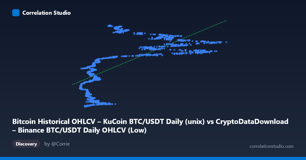
Bitcoin Historical OHLCV – KuCoin BTC/USDT Daily (unix) vs CryptoDataDownload – Binance BTC/USDT Daily OHLCV (Low)
- Pearson correlation (r)
- 0.6789
- Spearman correlation
- 0.7607
- p-value
- 0
- Sample size (n)
- 1861
- 95% confidence interval
- 0.6537 to 0.7027
- Granger causality
- None
- Granger optimal lag
- 10
AI analysis
Analysis: BTC/USDT Volume Column vs. Timestamp
Important initial observation: Before interpreting this as a meaningful "correlation," it's critical to note what these variables actually represent. The X-axis is a Unix timestamp (mislabeled in the data as an OHLCV column) and the Y-axis is also a timestamp-like value (1.5–1.67 billion range corresponds to Unix timestamps for 2017–2022 dates). This appears to be a data mapping issue — likely X represents a price/volume field and Y represents dates encoded as Unix time, or vice versa. Given the Y range (1,508,371,200 to 1,669,680,000) converts directly to calendar dates from October 2017 to November 2022, Y is functionally a time index, not an independent market variable. This reframes the entire analysis: we are likely looking at how some BTC metric (X) trends over time (Y), not a genuine bivariate market relationship.
1–2. Relationship Strength and Statistical Framing
With r = 0.679 and R² = 0.461, X explains about 46% of the variance in Y — a moderate-to-strong positive relationship, but leaving over half of the variance unexplained. The 95% CI [0.654, 0.703] is tight given the large sample (n=1,861), and the p-value of ~0 confirms the correlation is highly statistically significant and not due to chance. However, statistical significance here reflects the enormous sample size more than practical strength — R²=0.46 means this relationship has real but limited predictive value. The Granger causality results are telling: neither direction shows significant predictive causality (X→Y: p=0.84; Y→X: p=0.07, borderline). This strongly suggests the correlation is not a temporal lead-lag relationship but rather reflects both variables trending upward together over the sample period (likely because Y is essentially time itself, and X — probably price — has trended upward over 2017–2022).
3. Patterns and Outliers
The scatter shows a rough upward trend but with substantial scatter/heteroskedasticity: at low X values (~3,000–10,000), Y spans almost the entire timestamp range (2017–2022), while higher X values (40,000) cluster more tightly in 2021–2022 timestamps. This is consistent with X being BTC price: prices in the $3K–$10K range occurred across multiple periods (2018 bear market, 2020 pre-rally), while prices $40K only occurred in 2021–2022. This creates a "fan" or "wedge" shape rather than a clean linear band, explaining why R² is capped at 46% despite an obvious visual trend.
4. Confounding Factors and Caveats
The core caveat is that this is likely a spurious/mechanical correlation driven by shared trending behavior over time rather than a genuine causal or market relationship. Bitcoin price has a strong secular uptrend across 2017–2022 with high autocorrelation, and any variable that also trends (or is itself time-encoded) will show inflated correlation. Additionally, both series exhibit non-stationarity (trending, volatile), which violates assumptions needed for correlation/OLS to be meaningfully interpreted without differencing or detrending. The wide swings in BTC price (multiple bull/bear cycles) mean the relationship is likely non-linear and regime-dependent, not well captured by a single linear coefficient.
5. Recommendations
1. Clarify variable definitions — confirm what X and Y actually represent, since the Y-axis values are suspiciously date-like; this may be a data pipeline artifact rather than a genuine feature pair. 2. Detrend or difference both series (e.g., use daily returns instead of levels) before computing correlation to remove spurious trend-driven correlation. 3. Segment by market regime (bull/bear/sideways) to check if the relationship is stable or driven by specific periods (e.g., 2021 bull run). 4. Given the null Granger causality result, do not use this pair for predictive/forecasting purposes in its current form — the relationship is contemporaneous/structural, not lead-lag. 5. Re-run analysis with properly labeled, stationary variables (e.g., price vs. volume, or returns vs. volatility) to extract genuine market insight.
X dataset: CryptoDataDownload – Binance BTC/USDT Daily OHLCV
Y dataset: Bitcoin Historical OHLCV – KuCoin BTC/USDT Daily
Part of experiment: Bitcoin - CryptoDataDownload – Binance BTC/USDT Daily OHLCV vs Bitcoin Historical OHLCV – KuCoin BTC/USDT Daily