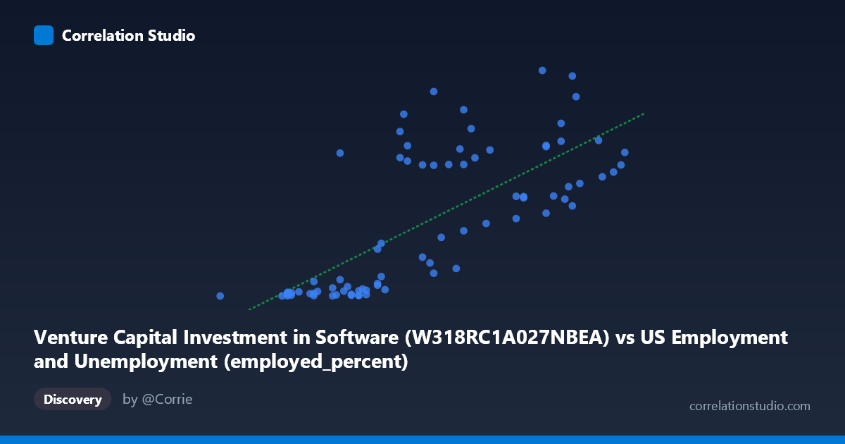
Venture Capital Investment in Software (W318RC1A027NBEA) vs US Employment and Unemployment (employed_percent)
- Pearson correlation (r)
- 0.7319
- Spearman correlation
- 0.7705
- p-value
- 0
- Sample size (n)
- 79
- 95% confidence interval
- 0.6094 to 0.8203
- Granger causality
- None
- Granger optimal lag
- 10
AI analysis
Scatterplot Analysis: Venture Capital Software Investment vs. Employment Percentage
Overview of the Relationship
The scatterplot reveals a positive relationship between Venture Capital Investment in Software (X-axis) and the employed percentage of the US labor force (Y-axis) across annual observations spanning 1946–2024. As software investment rises, employment percentage tends to increase as well. However, the scatter around the regression line (y = 38.437x − 2117.67) is substantial, indicating that while the trend is real and statistically meaningful, the relationship is far from deterministic. Notably, the axes appear to have been swapped in the dataset labels — venture capital software investment is plotted on X while employment percentage is on Y — which is worth keeping in mind when interpreting directionality.
Correlation Strength and Statistical Significance
The Pearson correlation of r = 0.732 indicates a moderately strong positive association. The R² of 0.536 means that approximately 53.6% of the variance in employment percentage is explained by software investment levels, leaving nearly half the variance attributable to other factors. The 95% confidence interval for r [0.609, 0.820] is relatively tight and entirely positive, reinforcing confidence that the true relationship is meaningfully positive rather than a sampling artifact. The p-value of 1.82 × 10⁻¹⁴ is extraordinarily small, confirming the correlation is highly statistically significant across 79 paired annual observations. However, Granger causality tests find no significant predictive direction in either direction (X→Y: F=1.67, p=0.115; Y→X: F=1.52, p=0.162), meaning that past values of software investment do not reliably forecast future employment levels, and vice versa. This is a critical caveat: correlation exists, but temporal predictive power is absent, suggesting both variables may be co-driven by a common underlying force (e.g., broader economic expansion cycles) rather than one causing the other.
Notable Patterns, Clusters, and Outliers
The data reveals at least two visually distinct clusters. A dense lower-left cluster groups many observations with X values between roughly 53.6–58.5 and Y values below ~50, suggesting an era of low software investment coinciding with lower or more modest employment percentages. A second, more dispersed upper-right cluster spans X values of ~58–64.4 with Y values ranging widely from ~40 to 466, indicating high variance in employment outcomes even at elevated investment levels. Several notable outliers are visible: the point near (62.2, 466.4) — the highest Y value — stands far above the regression line, as does (63.0, 455.0) and (58.5, 376.2), suggesting specific years where employment percentage spiked disproportionately relative to investment. Conversely, points like (57.1, 2.33) and (53.6, 0.85) anchor the low end. The non-linear appearance of the spread — with variance in Y expanding dramatically as X increases — hints at possible heteroscedasticity, suggesting a log or power transformation of Y might improve model fit.
Confounding Factors and Caveats
Several important caveats apply. First, this is an annual time-series correlation spanning nearly 80 years, meaning secular trends (long-run economic growth, technological transformation, population changes) likely drive both variables simultaneously, inflating the correlation without implying causation. This is precisely what the failed Granger causality tests suggest. Second, the dataset label descriptions appear internally inconsistent — the X-axis column is listed as coming from the "US Employment and Unemployment" dataset while the Y-axis comes from the "Venture Capital Investment in Software" dataset, suggesting a possible column assignment error that should be verified before drawing conclusions. Third, software investment figures and employment percentages are measured on entirely different scales and influenced by distinct policy, demographic, and macroeconomic forces — including Federal Reserve interest rate cycles, tax policy, immigration, and automation — none of which are controlled for here. The wide Y-axis spread at similar X values (e.g., Y ranging from ~2 to ~340 all near X=57–58) powerfully illustrates this residual unexplained variance.
Actionable Insights and Further Investigation
Given the strong correlation but absent Granger causality, the most productive next steps would include: (1) testing whether a log transformation of Y (employment percentage) linearizes the relationship and reduces heteroscedasticity, given the apparent funnel-shaped variance expansion; (2) introducing control variables such as GDP growth rate, federal funds rate, or total R&D spending to partial out shared macroeconomic trends and isolate any true independent effect; (3) verifying the axis-column assignment to ensure variables are correctly attributed to their respective datasets; (4) performing a structural break analysis to detect whether the relationship shifted post-2000 (dot-com boom), post-2008 (financial crisis), or post-2020 (pandemic-driven tech acceleration); and (5) disaggregating annual data into sub-periods to test whether the correlation is driven by a specific historical era rather than a stable, persistent relationship.
X dataset: US Employment and Unemployment
Y dataset: Venture Capital Investment in Software
Part of experiment: Yearly - US Employment and Unemployment vs Venture Capital Investment in Software